Figure S9. Validation of ColocBoost colocalization.

• S9a. Variant set-level excess-of-overlap (EOO) analysis of (i) 95% CoS-gene links from xQTL-only ColocBoost, (ii) standard marginal xQTL-gene associations, merged across all 17 xQTL datasets and (iii) 95% credible set (CS)-gene links from SuSiE fine-mapping, merged across all 17 xQTL datasets, against 118,389 regulatory element-gene maps from Promoter Capture Hi-C assay in the dorsolateral prefrontal cortex brain tissue, which profiles targeted 3D contacts linking gene promoters to proximal or distal regulatory elements.

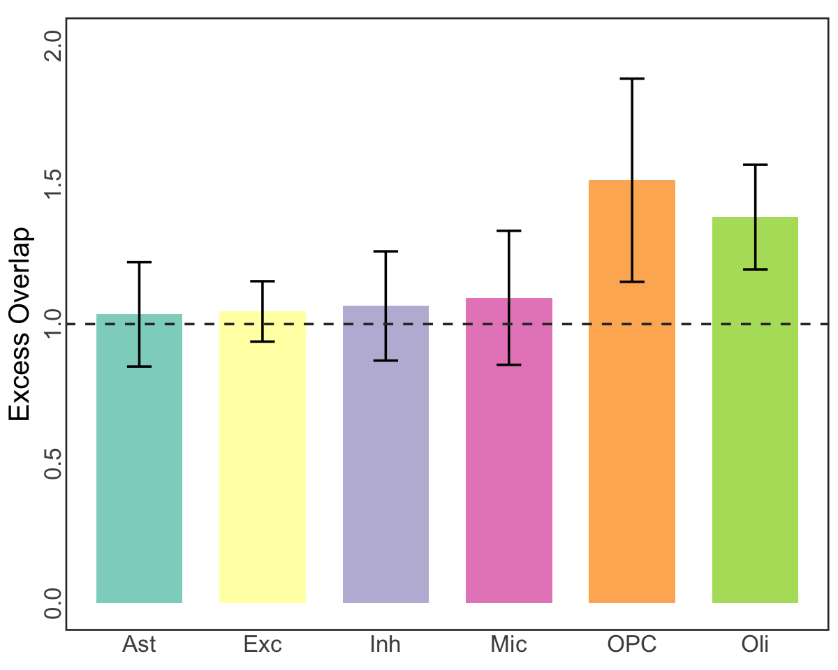
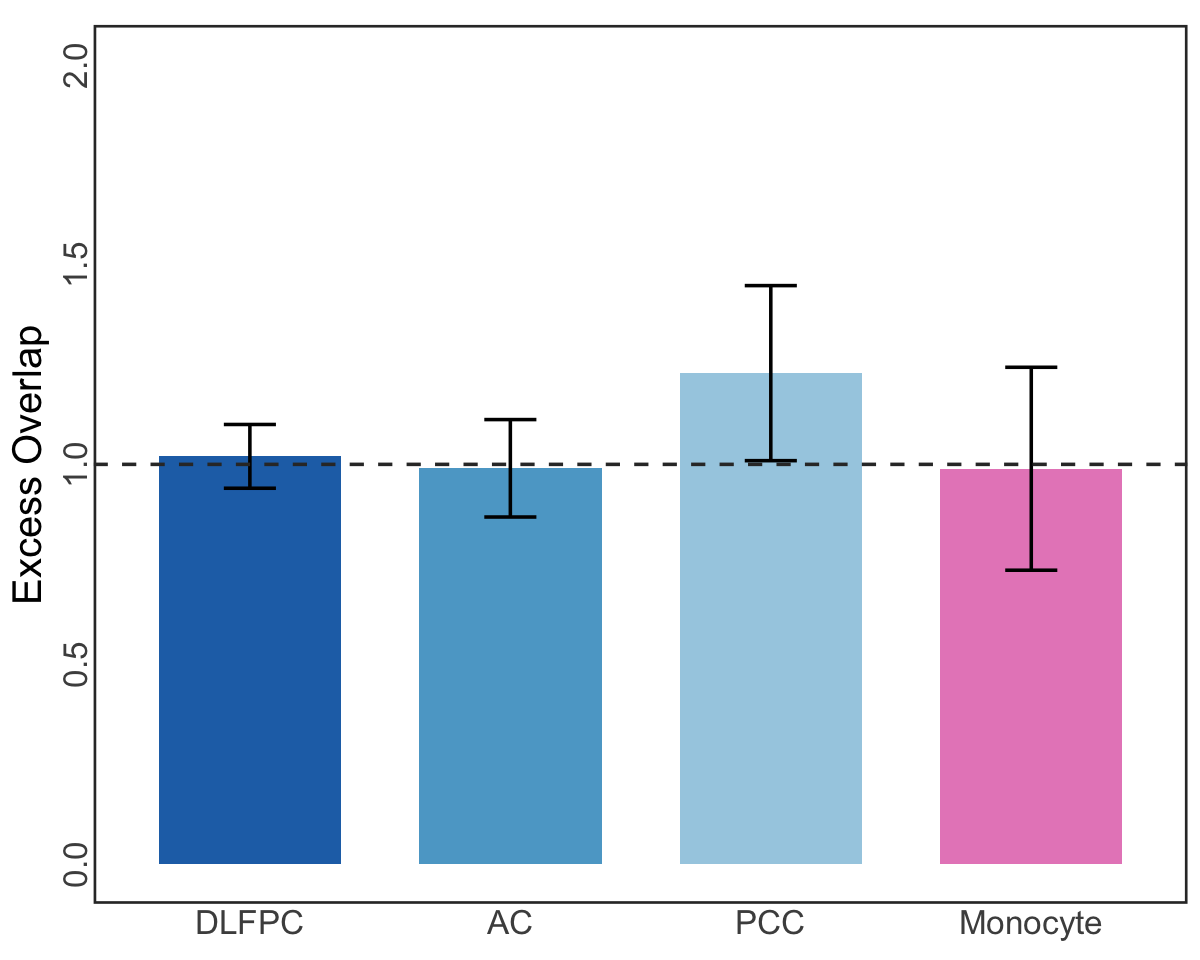
• S9b,c. EOO analysis of 95% CoS-gene links across (b) 3 different brain cortical regions and CD14+/CD16- bulk monocytes, and (c) 6 different brain cell types, against regulatory element-gene maps from PCHi-C data.

• S9d. Colocalization for SUOX in detail, also validated by CRIPRi in K562 cells. Error bars denote 95% confidence intervals. (See Figure4d)

Figure S9a

Variant set-level excess-of-overlap (EOO) analysis of (i) 95% CoS-gene links from xQTL-only ColocBoost, (ii) standard marginal xQTL-gene associations, merged across all 17 xQTL datasets and (iii) 95% credible set (CS)-gene links from SuSiE fine-mapping, merged across all 17 xQTL datasets, against 118,389 regulatory element-gene maps from Promoter Capture Hi-C assay in the dorsolateral prefrontal cortex brain tissue, which profiles targeted 3D contacts linking gene promoters to proximal or distal regulatory elements.

library(ggplot2)
library(ggsci)
sdtimes <- 1.96
data <- readRDS("Figure_S9a.rds")
p <- ggplot(data, aes(x = method, y = enrichment, fill = method)) +
  geom_bar(stat = "identity", width = 0.7, position = position_dodge(width = 0.9)) +
  geom_errorbar(aes(ymin = enrichment - sdtimes*sd, ymax = enrichment + sdtimes*sd), width = 0.2, position = position_dodge(0.7), linewidth = 1) +
  geom_text(
    data = subset(data, P <= 0.05/3 & enrichment > 0),
    aes(label = "*", y = enrichment + sdtimes * sd + 0.03),
    vjust = 0, color = "#F94144", size = 10, position = position_dodge(0.7)
  ) +
  # geom_text(data = subset(data, P <= 0.05/3), aes(label = "*", y = enrichment + sdtimes * sd + 0.03), vjust = 0, color = "#F94144", size = 6) +
  geom_hline(yintercept = 1, linetype = "dashed", color = "grey20", linewidth = 1)  + 
  scale_fill_brewer(palette = "Set1") +
  labs(
    title = "",
    x = "",
    y = "Excess Overlap"
  ) +
  ylim(c(0,20)) +
  theme_minimal(base_size = 15) +
  theme(
    plot.title = element_text(size = 0, face = "bold", hjust = 0.5),
    axis.title.x = element_text(size = 0),
    axis.title.y = element_text(size = 24),
    axis.text.y = element_text(size = 20, margin = margin(r = 0), angle = 90, hjust = 0.5, vjust = 0),
    axis.text.x = element_text(size = 20, margin = margin(t = 0)),
    legend.position = "none",
    panel.border = element_rect(color = "grey20", fill = NA, linewidth = 1.5)
  )

options(repr.plot.width = 8, repr.plot.height = 6)
p

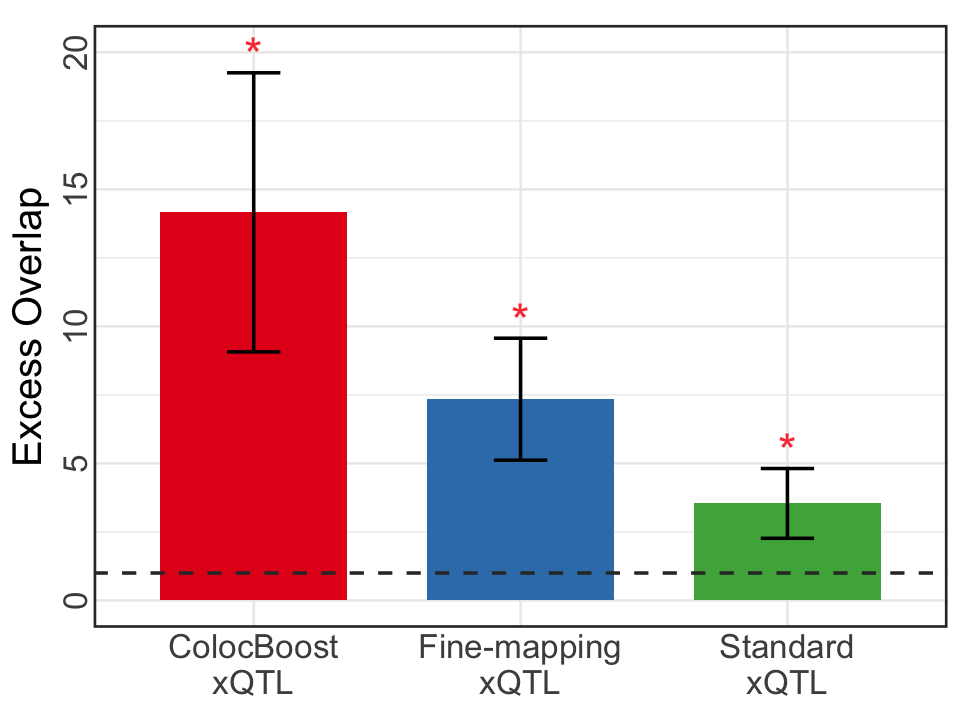
Figure S9b,c

EOO analysis of 95% CoS-gene links across (b) 3 different brain cortical regions and CD14+/CD16- bulk monocytes, and (c) 6 different brain cell types, against regulatory element-gene maps from PCHi-C data.

library(ggplot2)
library(ggsci)
data <- readRDS("Figure_S9b.rds")
sdtimes <- 1.96
colors <- c("#2171B5", "#5CA7CE", "#A6CEE3", "#E78AC3")
p1 <- ggplot(data, aes(x = celltype, y = enrichment, fill = celltype)) +
  geom_bar(stat = "identity", width = 0.7, position = position_dodge(width = 0.9)) +
  geom_errorbar(aes(ymin = enrichment - sdtimes*sd, ymax = enrichment + sdtimes*sd), width = 0.2, position = position_dodge(0.7), linewidth = 1) +
  geom_hline(yintercept = 1, linetype = "dashed", color = "grey20", linewidth = 1)  + 
  # scale_fill_brewer(palette = "Set3") +
  scale_fill_manual(values = colors) +
  labs(
    title = "",
    x = "",
    y = "Excess Overlap"
  ) +
  ylim(c(0,2)) +
  theme_minimal(base_size = 15) +
  theme(
    plot.title = element_text(size = 0, face = "bold", hjust = 0.5),
    axis.title.x = element_text(size = 0),
    axis.title.y = element_text(size = 24),
    axis.text.y = element_text(size = 20, margin = margin(r = 0), angle = 90, hjust = 0.5, vjust = 0),
    axis.text.x = element_text(size = 20, margin = margin(t = 0)),
    legend.position = "none",
    legend.title = element_text(size = 0),
    legend.text = element_text(size = 20),
    legend.spacing.y = unit(1.5, "cm"),
    panel.border = element_rect(color = "grey20", fill = NA, linewidth = 1.5),
    panel.grid.major = element_blank(),      # Remove major grid lines
    panel.grid.minor = element_blank(),      # Remove minor grid lines
  )

options(repr.plot.width = 10, repr.plot.height = 8)
p1

library(ggplot2)
library(ggsci)
data <- readRDS("Figure_S9c.rds")
sdtimes <- 1.96
colors <- c("#8DD3C7", "#FFFFB3", "#BEBADA", "#E78AC3", "#FDB462", "#B3DE69")
p2 <- ggplot(data, aes(x = celltype, y = enrichment, fill = celltype)) +
  geom_bar(stat = "identity", width = 0.7, position = position_dodge(width = 0.9)) +
  geom_errorbar(aes(ymin = enrichment - sdtimes*sd, ymax = enrichment + sdtimes*sd), width = 0.2, position = position_dodge(0.7), linewidth = 1) +
  geom_hline(yintercept = 1, linetype = "dashed", color = "grey20", linewidth = 1)  + 
  # scale_fill_brewer(palette = "Set3") +
  scale_fill_manual(values = colors) +
  labs(
    title = "",
    x = "",
    y = "Excess Overlap"
  ) +
  ylim(c(0,2)) +
  theme_minimal(base_size = 15) +
  theme(
    plot.title = element_text(size = 0, face = "bold", hjust = 0.5),
    axis.title.x = element_text(size = 0),
    axis.title.y = element_text(size = 24),
    axis.text.y = element_text(size = 20, margin = margin(r = 0), angle = 90, hjust = 0.5, vjust = 0),
    axis.text.x = element_text(size = 20, margin = margin(t = 0)),
    legend.position = "none",
    legend.title = element_text(size = 0),
    legend.text = element_text(size = 20),
    legend.spacing.y = unit(1.5, "cm"),
    panel.border = element_rect(color = "grey20", fill = NA, linewidth = 1.5),
    panel.grid.major = element_blank(),      # Remove major grid lines
    panel.grid.minor = element_blank(),      # Remove minor grid lines
  )

options(repr.plot.width = 10, repr.plot.height = 8)
p2