Figure 2b. Representative simulation examples.#
Representative simulation examples illustrating limitations of competing methods: (i) methods under “one-causal” assumption fail to detect causal signals with heterogeneous effects and (ii) spurious detection of non-causal variants with strongest marginal effect; (iii) COLOC (V5) shows reduced sensitivity to weak causal effects in GWAS.
1. Heterogeneous effects for two causal variants#
When analyzing multiple causal variants, it’s important to consider that they may exhibit heterogeneous effects across different contexts, populations, or individuals.
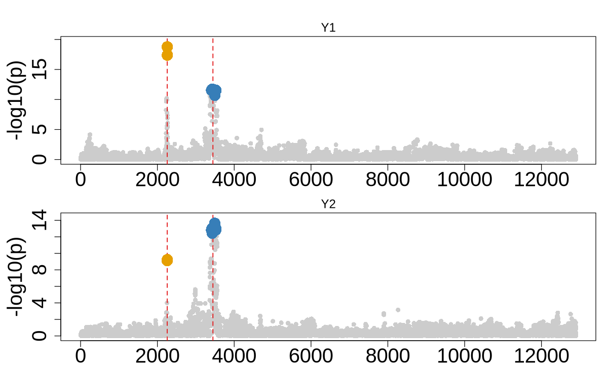
ColocBoost identify two CoS including two true causal variants.#
library(tidyverse)
library(colocboost)
load("data/Heterogeneous_Effect.rda")
data <- Heterogeneous_Effect
X <- data$X
Y <- data$Y
data$variant
── Attaching core tidyverse packages ──────────────────────── tidyverse 2.0.0 ──
✔ dplyr     1.1.4     ✔ readr     2.1.5
✔ forcats   1.0.0     ✔ stringr   1.5.1
✔ ggplot2   3.5.1     ✔ tibble    3.2.1
✔ lubridate 1.9.4     ✔ tidyr     1.3.1
✔ purrr     1.0.4
── Conflicts ────────────────────────────────────────── tidyverse_conflicts() ──
✖ dplyr::filter() masks stats::filter()
✖ dplyr::lag()    masks stats::lag()
ℹ Use the conflicted package (<http://conflicted.r-lib.org/>) to force all conflicts to become errors
- 622
- 1275
res <- colocboost(X = X, Y = Y)
res$cos_details$cos$cos_index
Starting checking the input data.

Starting gradient boosting algorithm.

Boosting iterations for outcome 1 converge after 51 iterations!

Boosting iterations for outcome 2 converge after 56 iterations!

Starting assemble analyses and results summary.
- $`cos1:y1_y2`
- 622
- $`cos2:y1_y2`
-
- 1293
- 1270
- 1288
- 1287
- 1305
- 1300
- 1275
- 1271
- 1273
- 1290
- 1291
options(repr.plot.width = 10, repr.plot.height = 6)
colocboost_plot(res, plot_cols = 1, add_vertical = T, add_vertical_idx = c(data$variant))
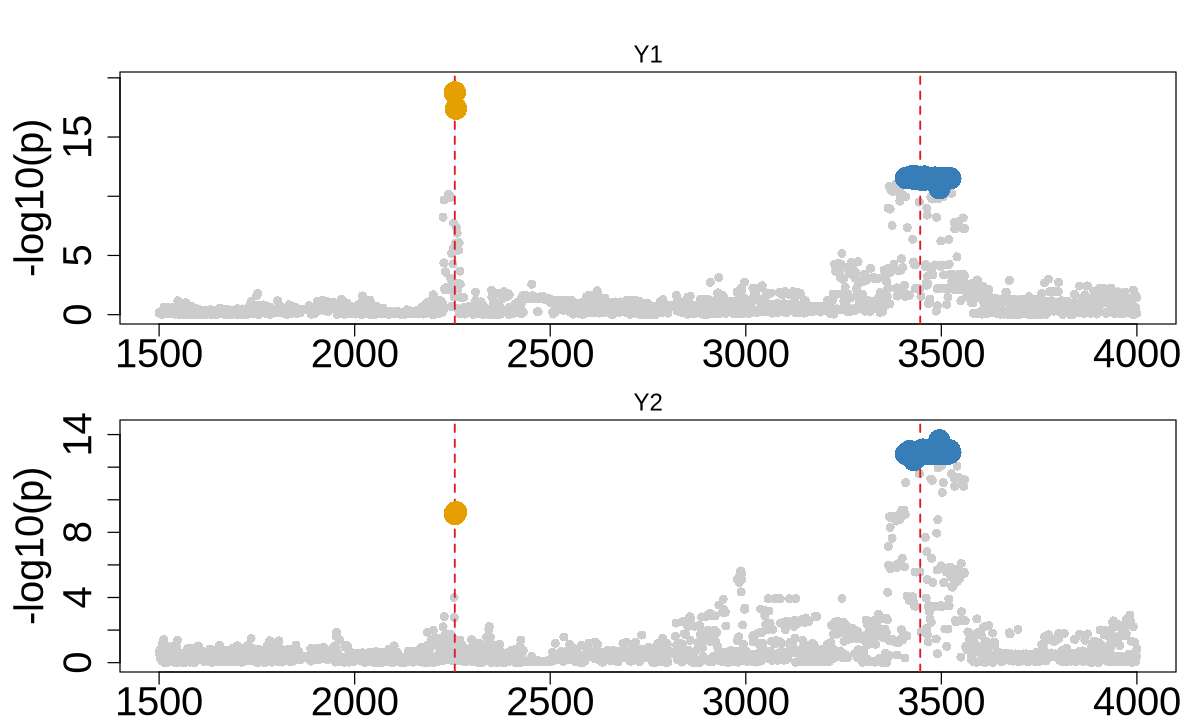
colocboost_plot(res, plot_cols = 1, add_vertical = T, add_vertical_idx = c(data$variant), grange = c(0:2000))
res$cos_details$cos_purity$min_abs_cor
| cos1:y1_y2 | cos2:y1_y2 | |
|---|---|---|
| cos1:y1_y2 | 0.9869088 | 0.0125171 |
| cos2:y1_y2 | 0.0125171 | 0.9840258 |
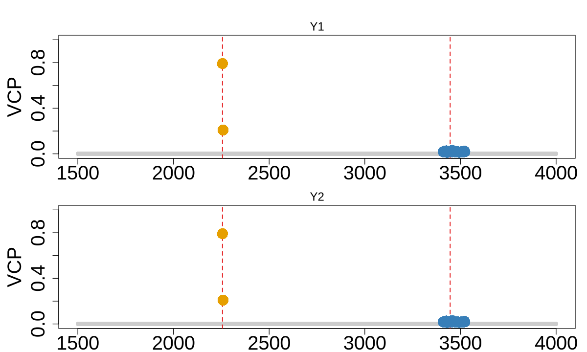
colocboost_plot(res, y = "vcp", plot_cols = 1, add_vertical = T, add_vertical_idx = c(data$variant),
                grange = c(0:2000))
HyPrColoc#
library(hyprcoloc)
betas = sebetas = matrix(NA, nrow = ncol(X), ncol = 2)
for (i in 1:2){
    x <- scale(X)
    y <- scale(Y[,i])
    rr <- susieR::univariate_regression(x, y)
    betas[,i] = rr$betahat
    sebetas[, i] <- rr$sebetahat
}
traits <- c(1:2)
rsid <- paste0("snp", c(1:ncol(X)))
colnames(betas) <- colnames(sebetas) <- traits
rownames(betas) <- rownames(sebetas) <- rsid
res_hyprcoloc <- hyprcoloc(betas, sebetas, trait.names=traits, snp.id=rsid, snpscores = TRUE)
Warning message:
“replacing previous import ‘Matrix::tcrossprod’ by ‘Rmpfr::tcrossprod’ when loading ‘hyprcoloc’”
Warning message:
“replacing previous import ‘Matrix::crossprod’ by ‘Rmpfr::crossprod’ when loading ‘hyprcoloc’”
Warning message:
“replacing previous import ‘Matrix::.__C__atomicVector’ by ‘Rmpfr::.__C__atomicVector’ when loading ‘hyprcoloc’”
res_hyprcoloc$results
| iteration | traits | posterior_prob | regional_prob | candidate_snp | posterior_explained_by_snp | dropped_trait |
|---|---|---|---|---|---|---|
| <dbl> | <chr> | <lgl> | <dbl> | <lgl> | <dbl> | <chr> |
| 1 | None | NA | 1 | NA | NA | 1 |
res_hyprcoloc %>% str
List of 1
 $ results:'data.frame':	1 obs. of  7 variables:
  ..$ iteration                 : num 1
  ..$ traits                    : chr "None"
  ..$ posterior_prob            : logi NA
  ..$ regional_prob             : num 1
  ..$ candidate_snp             : logi NA
  ..$ posterior_explained_by_snp: num NA
  ..$ dropped_trait             : chr "1"
 - attr(*, "class")= chr "hyprcoloc"
COLOC (one causal assumption)#
library(coloc)
LD <- get_cormat(X)
colnames(LD) <- rownames(LD) <- 1:ncol(X)
MAF <- colMeans(X)/2 %>% as.numeric
D1 <- list("beta" = betas[,1], "varbeta" = sebetas[,1]^2,
           "N" = nrow(X), "sdY" = sd(unlist(data$Y[,1])),
           "type" = 'quant', "MAF" = MAF, "LD" = LD,
           "snp" = 1:ncol(X), "position" = 1:ncol(X))
D2 <- list("beta" = betas[,2], "varbeta" = sebetas[,2]^2,
           "N" = nrow(X), "sdY" = sd(unlist(data$Y[,2])),
           "type" = 'quant', "MAF" = MAF, "LD" = LD,
           "snp" = 1:ncol(X), "position" = 1:ncol(X))
my.res <- coloc.abf(dataset1=D1, dataset2=D2)
This is coloc version 5.2.3

Warning message in adjust_prior(p1, nrow(df1), "1"):
“p1 * nsnps >= 1, setting p1=1/(nsnps + 1)”
Warning message in adjust_prior(p2, nrow(df2), "2"):
“p2 * nsnps >= 1, setting p2=1/(nsnps + 1)”
PP.H0.abf PP.H1.abf PP.H2.abf PP.H3.abf PP.H4.abf
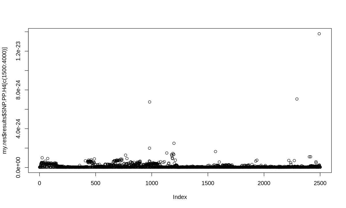
1.76e-21 4.33e-09 4.04e-13 9.93e-01 6.84e-03
[1] "PP abf for shared variant: 0.684%"
plot(my.res$results$SNP.PP.H4[c(1500:4000)])
COLOC (V5)#
library(susieR)
out_p <- runsusie(D1)
out_e <- runsusie(D2)
out_coloc = coloc.susie(out_e, out_p)
running max iterations: 100

	converged: TRUE

running max iterations: 100

	converged: TRUE
out_coloc$summary
| nsnps | hit1 | hit2 | PP.H0.abf | PP.H1.abf | PP.H2.abf | PP.H3.abf | PP.H4.abf | idx1 | idx2 |
|---|---|---|---|---|---|---|---|---|---|
| <int> | <chr> | <chr> | <dbl> | <dbl> | <dbl> | <dbl> | <dbl> | <int> | <int> |
| 12900 | 3495 | 2256 | 4.890181e-21 | 1.140795e-12 | 4.286644e-09 | 0.999999996 | 2.924359e-11 | 1 | 1 |
| 12900 | 2256 | 2256 | 9.904029e-19 | 4.439301e-15 | 8.681693e-07 | 0.001895203 | 9.981039e-01 | 2 | 1 |
| 12900 | 3495 | 3408 | 1.921831e-17 | 4.483300e-09 | 5.255216e-10 | 0.120836772 | 8.791632e-01 | 1 | 2 |
| 12900 | 2256 | 3408 | 8.156886e-12 | 3.656176e-08 | 2.230487e-04 | 0.999775096 | 1.818970e-06 | 2 | 2 |
o <- order(out_coloc$results$SNP.PP.H4.row2,decreasing=TRUE)
cs <- cumsum(out_coloc$results$SNP.PP.H4.row2[o])
w <- which(cs > 0.95)[1]
cos1 <- out_coloc$results[o,][1:w,]$snp
cos1
'2256'
o <- order(out_coloc$results$SNP.PP.H4.row3,decreasing=TRUE)
cs <- cumsum(out_coloc$results$SNP.PP.H4.row3[o])
w <- which(cs > 0.95)[1]
cos2 <- out_coloc$results[o,][1:w,]$snp
cos2
- '3425'
- '3426'
- '3457'
- '3521'
- '3419'
- '3480'
- '3453'
- '3437'
- '3495'
- '3416'
- '3484'
- '3523'
- '3410'
- '3411'
- '3414'
- '3415'
- '3417'
- '3420'
- '3421'
- '3422'
- '3423'
- '3424'
- '3432'
- '3435'
- '3439'
- '3440'
- '3449'
- '3450'
- '3451'
- '3452'
- '3454'
- '3455'
- '3456'
- '3458'
- '3472'
- '3476'
- '3479'
- '3481'
- '3482'
- '3485'
- '3486'
- '3504'
- '3508'
- '3510'
- '3511'
- '3512'
- '3516'
- '3447'
- '3446'
- '3494'
- '3428'
- '3438'
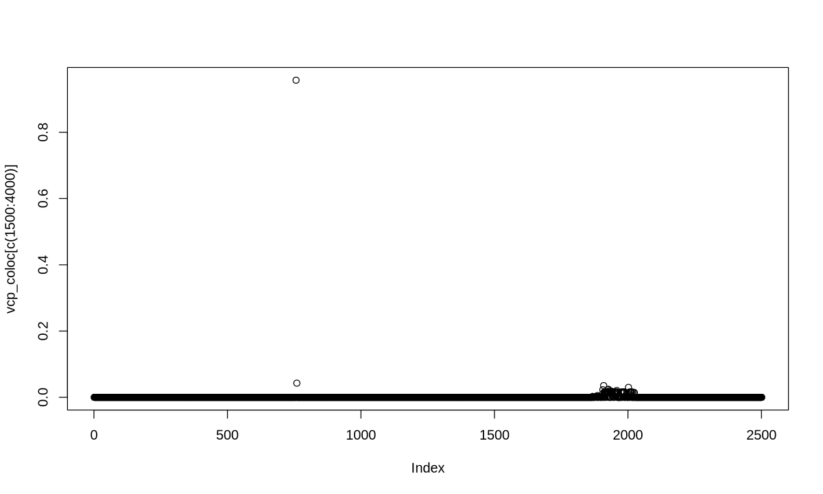
vcp_coloc <- 1 - (1-out_coloc$results$SNP.PP.H4.row1)*(1-out_coloc$results$SNP.PP.H4.row4)
plot(vcp_coloc[c(1500:4000)])
MOLOC#
library(moloc)
moloc_input <- lapply(1:2, function(cnt){
    tibble(SNP = 1:ncol(data$X), BETA = betas[,cnt],
           SE = sebetas[,cnt], N = nrow(data$X), MAF = MAF)
})
res_moloc <- moloc_test(listData = moloc_input)
Use default priors: 1e-04,1e-05

Mean estimated sdY from data1: 0.560918402515816

Mean estimated sdY from data2: 0.561003724043599

Use prior variances of 0.01 0.1 0.5

Use prior variances of 0.01 0.1 0.5

Best SNP per trait a: 2256

Probability that trait a colocalizes with at least one other trait = 0.0067

Best SNP per trait b: 2256

Probability that trait b colocalizes with at least one other trait = 0.0067

Best SNP per trait ab: 2256

Probability that trait ab colocalizes with at least one other trait = 0.0067
res_moloc$priors_lkl_ppa
| prior | sumbf | logBF_locus | PPA | |
|---|---|---|---|---|
| <dbl> | <dbl> | <dbl> | <dbl> | |
| a | 1.00e-04 | 37.56061 | 28.09563 | 4.648440e-09 |
| a,b | 1.00e-08 | 65.95099 | 47.02103 | 9.933272e-01 |
| b | 1.00e-04 | 28.39039 | 18.92540 | 4.838694e-13 |
| ab | 1.00e-05 | 54.04022 | 44.57524 | 6.672820e-03 |
| zero | 9.99e-01 | 0.00000 | 0.00000 | 2.264332e-21 |
res_moloc$best_snp
| coloc_ppas | best.snp.coloc | |
|---|---|---|
| <dbl> | <chr> | |
| a | 0.00667282 | 2256 |
| b | 0.00667282 | 2256 |
| ab | 0.00667282 | 2256 |
2. Non-causal strongest marginal effect#
library(colocboost)
library(tidyverse)
load("data/Non_Causal_Strongest_Marginal.rda")
data <- Non_Causal_Strongest_Marginal
X <- data$X
Y <- data$Y
data$variant
- 654
- 858
res <- colocboost(X = X, Y = Y)
res$cos_details$cos$cos_index
Starting checking the input data.

Starting gradient boosting algorithm.

Boosting iterations for outcome 1 converge after 50 iterations!

Boosting iterations for outcome 2 converge after 56 iterations!

Starting assemble analyses and results summary.
- $`cos1:y1_y2`
-
- 654
- 721
- 761
- 797
- 673
- 677
- 756
- 720
- 740
- 678
- 773
- 777
- $`cos2:y1_y2`
-
- 858
- 865
- 851
- 886
- 876
- 854
- 885
options(repr.plot.width = 10, repr.plot.height = 6)
colocboost_plot(res, plot_cols = 1, add_vertical = T, add_vertical_idx = c(data$variant))

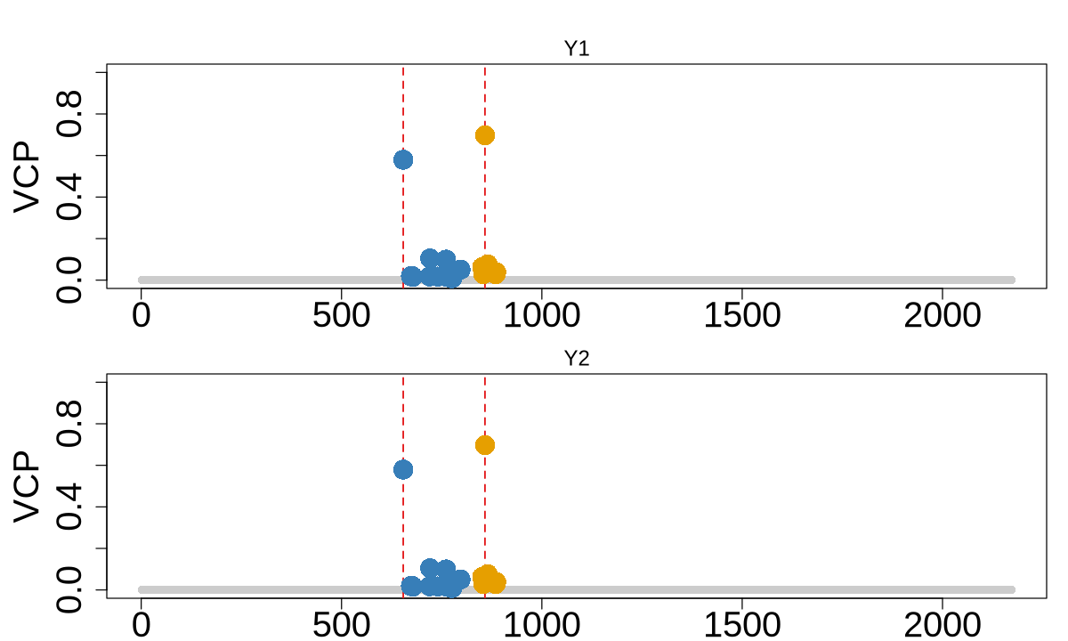
colocboost_plot(res, y = "vcp", plot_cols = 1, add_vertical = T, add_vertical_idx = c(data$variant))
res$cos_details$cos_purity$min_abs_cor
| cos1:y1_y2 | cos2:y1_y2 | |
|---|---|---|
| cos1:y1_y2 | 0.8666675 | 0.2562119 |
| cos2:y1_y2 | 0.2562119 | 0.7613753 |
HyPrColoc#
library(hyprcoloc)
betas = sebetas = matrix(NA, nrow = ncol(X), ncol = 2)
for (i in 1:2){
    x <- scale(X)
    y <- scale(Y[,i])
    rr <- susieR::univariate_regression(x, y)
    betas[,i] = rr$betahat
    sebetas[, i] <- rr$sebetahat
}
traits <- c(1:2)
rsid <- paste0("snp", c(1:ncol(X)))
colnames(betas) <- colnames(sebetas) <- traits
rownames(betas) <- rownames(sebetas) <- rsid
res_hyprcoloc <- hyprcoloc(betas, sebetas, trait.names=traits, snp.id=rsid, snpscores = TRUE)
res_hyprcoloc$results
| iteration | traits | posterior_prob | regional_prob | candidate_snp | posterior_explained_by_snp | dropped_trait |
|---|---|---|---|---|---|---|
| <dbl> | <chr> | <dbl> | <dbl> | <chr> | <dbl> | <lgl> |
| 1 | 1, 2 | 0.9995 | 1 | snp721 | 1 | NA |
plot(res_hyprcoloc$snpscores[[1]])

COLOC (one causal assumption)#
library(coloc)
LD <- get_cormat(data$X)
colnames(LD) <- rownames(LD) <- 1:ncol(data$X)
MAF <- colMeans(data$X)/2 %>% as.numeric
D1 <- list("beta" = betas[,1], "varbeta" = sebetas[,1]^2,
           "N" = nrow(data$X), "sdY" = sd(unlist(data$Y[,1])),
           "type" = 'quant', "MAF" = MAF, "LD" = LD,
           "snp" = 1:ncol(data$X), "position" = 1:ncol(data$X))
D2 <- list("beta" = betas[,2], "varbeta" = sebetas[,2]^2,
           "N" = nrow(data$X), "sdY" = sd(unlist(data$Y[,2])),
           "type" = 'quant', "MAF" = MAF, "LD" = LD,
           "snp" = 1:ncol(data$X), "position" = 1:ncol(data$X))
my.res <- coloc.abf(dataset1=D1, dataset2=D2)
PP.H0.abf PP.H1.abf PP.H2.abf PP.H3.abf PP.H4.abf
 6.41e-51  2.21e-28  3.44e-26  1.86e-04  1.00e+00
[1] "PP abf for shared variant: 100%"
o <- order(my.res$results$SNP.PP.H4,decreasing=TRUE)
cs <- cumsum(my.res$results$SNP.PP.H4[o])
w <- which(cs > 0.95)[1]
my.res$results[o,][1:w,]$snp
'721'
pph4.snp <- my.res$results$SNP.PP.H4[order(my.res$results$position,decreasing=FALSE)]
plot(pph4.snp[c(400:1200)])

COLOC (V5)#
library(susieR)
out_p <- runsusie(D1)
out_e <- runsusie(D2)
out_coloc = coloc.susie(out_e, out_p)
running max iterations: 100

	converged: TRUE

running max iterations: 100

	converged: TRUE
out_coloc$summary
o <- order(out_coloc$results$SNP.PP.H4.row2,decreasing=TRUE)
cs <- cumsum(out_coloc$results$SNP.PP.H4.row2[o])
w <- which(cs > 0.95)[1]
cos1 <- out_coloc$results[o,][1:w,]$snp
cos1
- '654'
- '721'
- '761'
- '673'
- '677'
- '797'
o <- order(out_coloc$results$SNP.PP.H4.row3,decreasing=TRUE)
cs <- cumsum(out_coloc$results$SNP.PP.H4.row3[o])
w <- which(cs > 0.95)[1]
cos2 <- out_coloc$results[o,][1:w,]$snp
cos2
'858'
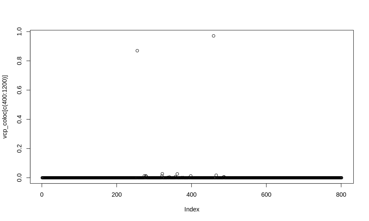
vcp_coloc <- 1 - (1-out_coloc$results$SNP.PP.H4.row2)*(1-out_coloc$results$SNP.PP.H4.row3)
plot(vcp_coloc[c(400:1200)])
MOLOC#
library(moloc)
moloc_input <- lapply(1:2, function(cnt){
    tibble(SNP = 1:ncol(data$X), BETA = betas[,cnt],
           SE = sebetas[,cnt], N = nrow(data$X), MAF = MAF)
})
res_moloc <- moloc_test(listData = moloc_input)
Use default priors: 1e-04,1e-05

Mean estimated sdY from data1: 0.553434902059988

Mean estimated sdY from data2: 0.553187001637554

Use prior variances of 0.01 0.1 0.5

Use prior variances of 0.01 0.1 0.5

Best SNP per trait a: 721

Probability that trait a colocalizes with at least one other trait = 1

Best SNP per trait b: 721

Probability that trait b colocalizes with at least one other trait = 1

Best SNP per trait ab: 721

Probability that trait ab colocalizes with at least one other trait = 1
res_moloc$priors_lkl_ppa
| prior | sumbf | logBF_locus | PPA | |
|---|---|---|---|---|
| <dbl> | <dbl> | <dbl> | <dbl> | |
| a | 1.00e-04 | 60.59171 | 52.90784 | 2.492328e-28 |
| a,b | 1.00e-08 | 125.07877 | 109.71104 | 2.529180e-04 |
| b | 1.00e-04 | 65.56983 | 57.88597 | 3.618911e-26 |
| ab | 1.00e-05 | 126.45320 | 118.76934 | 9.997471e-01 |
| zero | 9.99e-01 | 0.00000 | 0.00000 | 1.207708e-50 |
res_moloc$best_snp
| coloc_ppas | best.snp.coloc | |
|---|---|---|
| <dbl> | <chr> | |
| a | 0.9997471 | 721 |
| b | 0.9997471 | 721 |
| ab | 0.9997471 | 721 |
3. Weaker causal effect for target traits#
library(colocboost)
library(tidyverse)
load("data/Weaker_GWAS_Effect.rda")
data <- Weaker_GWAS_Effect
X <- data$X
Y <- data$Y
data$variant
- 1926
- 2271
res <- colocboost(X = X, Y = Y)
res$cos_details$cos$cos_index
Starting checking the input data.

Starting gradient boosting algorithm.

Boosting iterations for outcome 1 converge after 23 iterations!

Boosting iterations for outcome 2 converge after 33 iterations!

Starting assemble analyses and results summary.
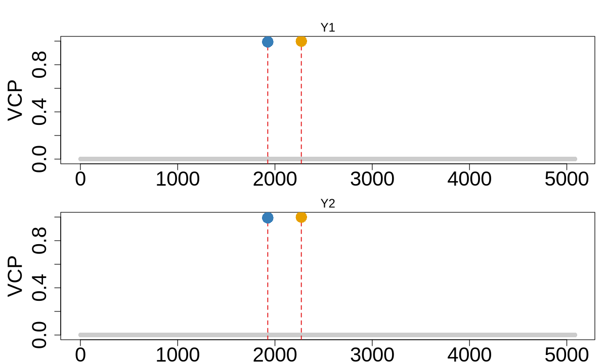
- $`cos1:y1_y2`
- 1926
- $`cos2:y1_y2`
- 2271
options(repr.plot.width = 10, repr.plot.height = 6)
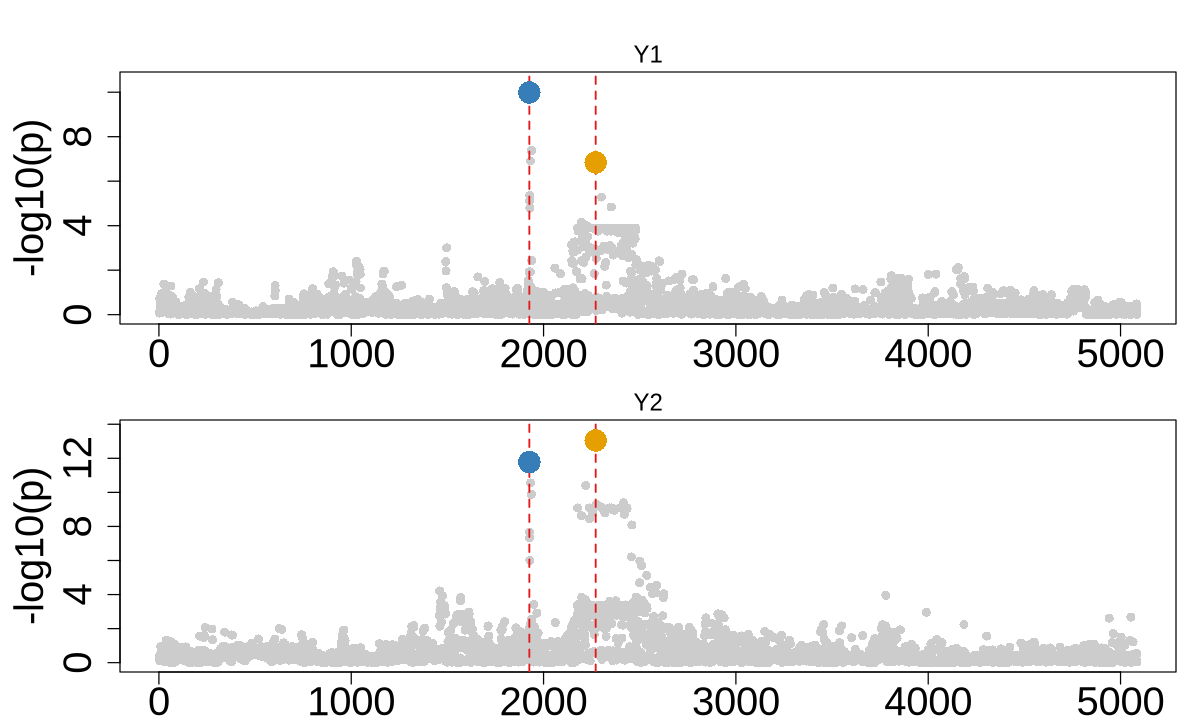
colocboost_plot(res, plot_cols = 1, add_vertical = T, add_vertical_idx = c(data$variant))
colocboost_plot(res, y = "vcp", plot_cols = 1, add_vertical = T, add_vertical_idx = c(data$variant))
HyPrColoc#
library(hyprcoloc)
betas = sebetas = matrix(NA, nrow = ncol(X), ncol = 2)
for (i in 1:2){
x <- scale(X)
y <- scale(Y[,i])
rr <- susieR::univariate_regression(x, y)
betas[,i] = rr$betahat
sebetas[, i] <- rr$sebetahat
}
traits <- c(1:2)
rsid <- paste0("snp", c(1:ncol(X)))
colnames(betas) <- colnames(sebetas) <- traits
rownames(betas) <- rownames(sebetas) <- rsid
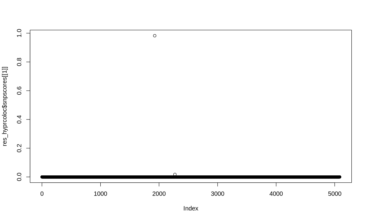
res_hyprcoloc <- hyprcoloc(betas, sebetas, trait.names=traits, snp.id=rsid, snpscores = TRUE)
res_hyprcoloc$results
| iteration | traits | posterior_prob | regional_prob | candidate_snp | posterior_explained_by_snp | dropped_trait |
|---|---|---|---|---|---|---|
| <dbl> | <chr> | <dbl> | <dbl> | <chr> | <dbl> | <lgl> |
| 1 | 1, 2 | 0.9616 | 1 | snp1926 | 0.9823 | NA |
plot(res_hyprcoloc$snpscores[[1]])
COLOC (one causal assumption)#
library(coloc)
LD <- get_cormat(data$X)
colnames(LD) <- rownames(LD) <- 1:ncol(data$X)
MAF <- colMeans(data$X)/2 %>% as.numeric
D1 <- list("beta" = betas[,1], "varbeta" = sebetas[,1]^2,
           "N" = nrow(data$X), "sdY" = sd(unlist(data$Y[,1])),
           "type" = 'quant', "MAF" = MAF, "LD" = LD,
           "snp" = 1:ncol(data$X), "position" = 1:ncol(data$X))
D2 <- list("beta" = betas[,2], "varbeta" = sebetas[,2]^2,
           "N" = nrow(data$X), "sdY" = sd(unlist(data$Y[,2])),
           "type" = 'quant', "MAF" = MAF, "LD" = LD,
           "snp" = 1:ncol(data$X), "position" = 1:ncol(data$X))
my.res <- coloc.abf(dataset1=D1, dataset2=D2)
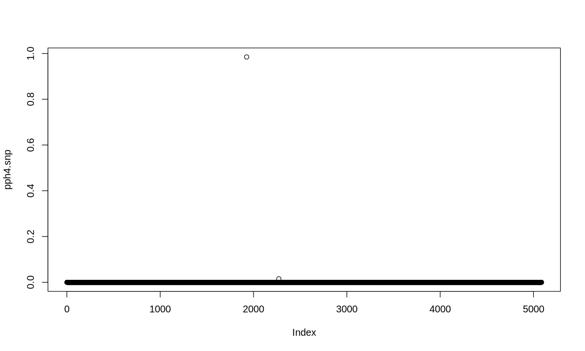
PP.H0.abf PP.H1.abf PP.H2.abf PP.H3.abf PP.H4.abf
 3.94e-13  2.65e-09  2.69e-06  1.71e-02  9.83e-01
[1] "PP abf for shared variant: 98.3%"
o <- order(my.res$results$SNP.PP.H4,decreasing=TRUE)
cs <- cumsum(my.res$results$SNP.PP.H4[o])
w <- which(cs > 0.95)[1]
my.res$results[o,][1:w,]$snp
'1926'
pph4.snp <- my.res$results$SNP.PP.H4[order(my.res$results$position,decreasing=FALSE)]
plot(pph4.snp)
COLOC (V5)#
library(susieR)
out_p <- runsusie(D1)
out_e <- runsusie(D2)
out_coloc = coloc.susie(out_e, out_p)
running max iterations: 100

	converged: TRUE

running max iterations: 100

	converged: TRUE
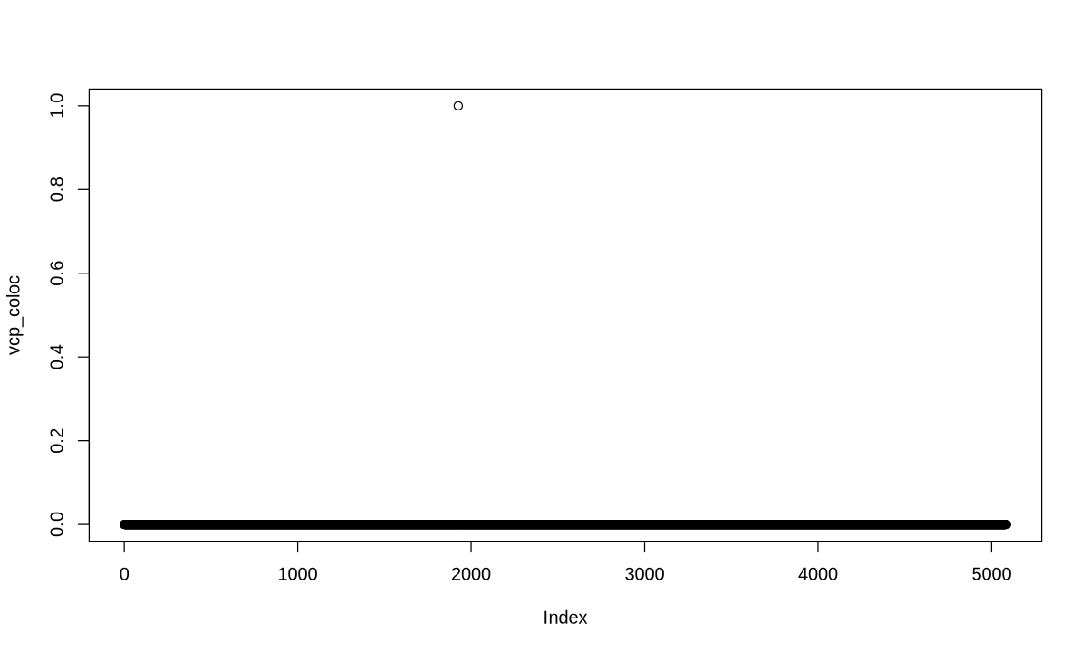
out_coloc$summary
o <- order(out_coloc$results$SNP.PP.H4.row2,decreasing=TRUE)
cs <- cumsum(out_coloc$results$SNP.PP.H4.row2[o])
w <- which(cs > 0.95)[1]
cos1 <- out_coloc$results[o,][1:w,]$snp
cos1
'1926'
vcp_coloc <- out_coloc$results$SNP.PP.H4.row2
plot(vcp_coloc)
MOLOC#
library(moloc)
moloc_input <- lapply(1:2, function(cnt){
    tibble(SNP = 1:ncol(data$X), BETA = betas[,cnt],
           SE = sebetas[,cnt], N = nrow(data$X), MAF = MAF)
})
res_moloc <- moloc_test(listData = moloc_input)
Use default priors: 1e-04,1e-05

Mean estimated sdY from data1: 0.537763795330779

Mean estimated sdY from data2: 0.537609105700604

Use prior variances of 0.01 0.1 0.5

Use prior variances of 0.01 0.1 0.5

Best SNP per trait a: 1926

Probability that trait a colocalizes with at least one other trait = 0.99

Best SNP per trait b: 1926

Probability that trait b colocalizes with at least one other trait = 0.99

Best SNP per trait ab: 1926

Probability that trait ab colocalizes with at least one other trait = 0.99
res_moloc$priors_lkl_ppa
| prior | sumbf | logBF_locus | PPA | |
|---|---|---|---|---|
| <dbl> | <dbl> | <dbl> | <dbl> | |
| a | 1.00e-04 | 17.99025 | 9.456204 | 1.984014e-09 |
| a,b | 1.00e-08 | 42.71907 | 25.650974 | 1.089268e-02 |
| b | 1.00e-04 | 24.81574 | 16.281686 | 1.827317e-06 |
| ab | 1.00e-05 | 40.32003 | 31.785978 | 9.891055e-01 |
| zero | 9.99e-01 | 0.00000 | 0.000000 | 3.051242e-13 |
res_moloc$best_snp
| coloc_ppas | best.snp.coloc | |
|---|---|---|
| <dbl> | <chr> | |
| a | 0.9891055 | 1926 |
| b | 0.9891055 | 1926 |
| ab | 0.9891055 | 1926 |