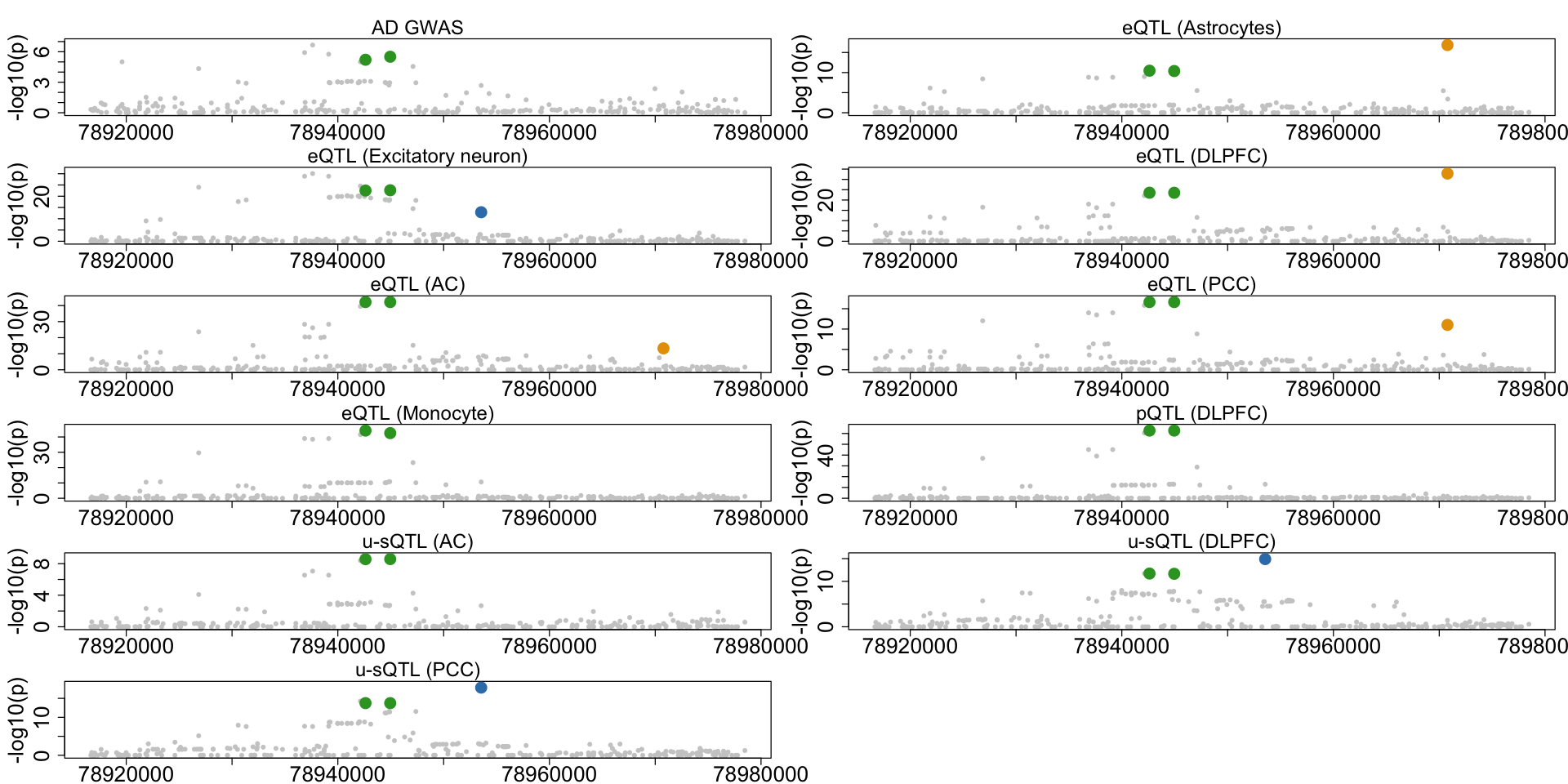
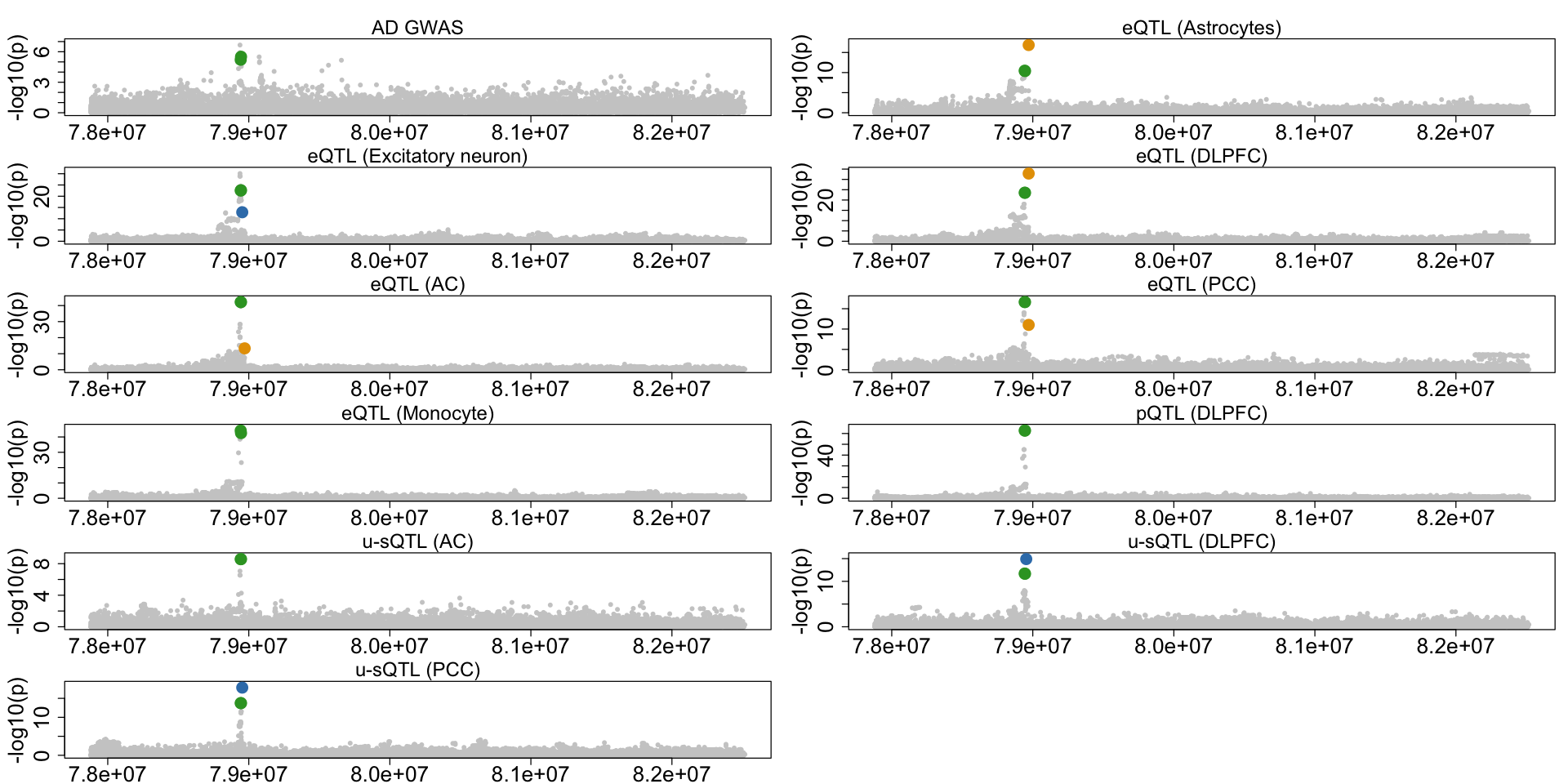
Figure 6h. Colocalization across multiple xQTLs in CTSH.#
A second example case of AD-xQTL colocalization demonstrating three distinct CoS showing different colocalization patterns across multiple brain cell types for the CTSH gene.
for(file in list.files("/Users/xueweic/Documents/GitHub/statfungen/colocboost/R", full.names = T)) {source(file)}
res <- readRDS("data/Figure_6h_CTSH.rds")
options(repr.plot.width = 16, repr.plot.height = 8)
outcome_names <- c("Mic", "eQTL (Astrocytes)", "Oli", "eQTL (Excitatory neuron)",
                  "Inh", "eQTL (DLPFC)", "eQTL (AC)", "eQTL (PCC)", "eQTL (Monocyte)",
                  "pQTL (DLPFC)", "u-sQTL (AC)", "p-sQTL (DLPFC)", "u-sQTL (DLPFC)",
                  "p-sQTL (PCC)", "u-sQTL (PCC)", "AD GWAS")
colocboost_plot(res, outcome_names = outcome_names, variant_coord = TRUE, plot_cols = 2)
res$cos_details$cos_outcomes_npc
- $`cos1:y4_y13_y15`
A data.frame: 3 × 3 outcomes_index relative_logLR npc_outcome <int> <dbl> <dbl> PCC_unproductive 15 2.396364046 0.991710189 DLPFC_unproductive 13 2.115126649 0.985451295 Exc 4 0.002061726 0.004114962 - $`cos2:y2_y6_y7_y8`
A data.frame: 4 × 3 outcomes_index relative_logLR npc_outcome <dbl> <dbl> <dbl> DLPFC 6 5.675018 0.9999882 Ast 2 2.696527 0.9954519 AC 7 2.148031 0.9863779 PCC 8 1.803699 0.9728777 - $`cos3:y2_y4_y6_y7_y8_y9_y10_y11_y13_y15_y16`
A data.frame: 11 × 3 outcomes_index relative_logLR npc_outcome <dbl> <dbl> <dbl> pQTL 10 7.54702741 0.9999997 AC 7 6.61211940 0.9999982 Monocyte 9 4.16130551 0.9997570 DLPFC 6 3.80459620 0.9995041 PCC 8 2.56381706 0.9940694 Ast 2 1.21139561 0.9113262 AC_unproductive 11 0.88435923 0.8294486 DLPFC_unproductive 13 0.85215225 0.8181011 PCC_unproductive 15 0.85128304 0.8177847 ADGWAS 16 0.41501195 0.5639611 Exc 4 0.05393756 0.1022603
colocboost_plot(res, pos = c(5650:5950), outcome_names = outcome_names, variant_coord = TRUE, plot_cols = 2)