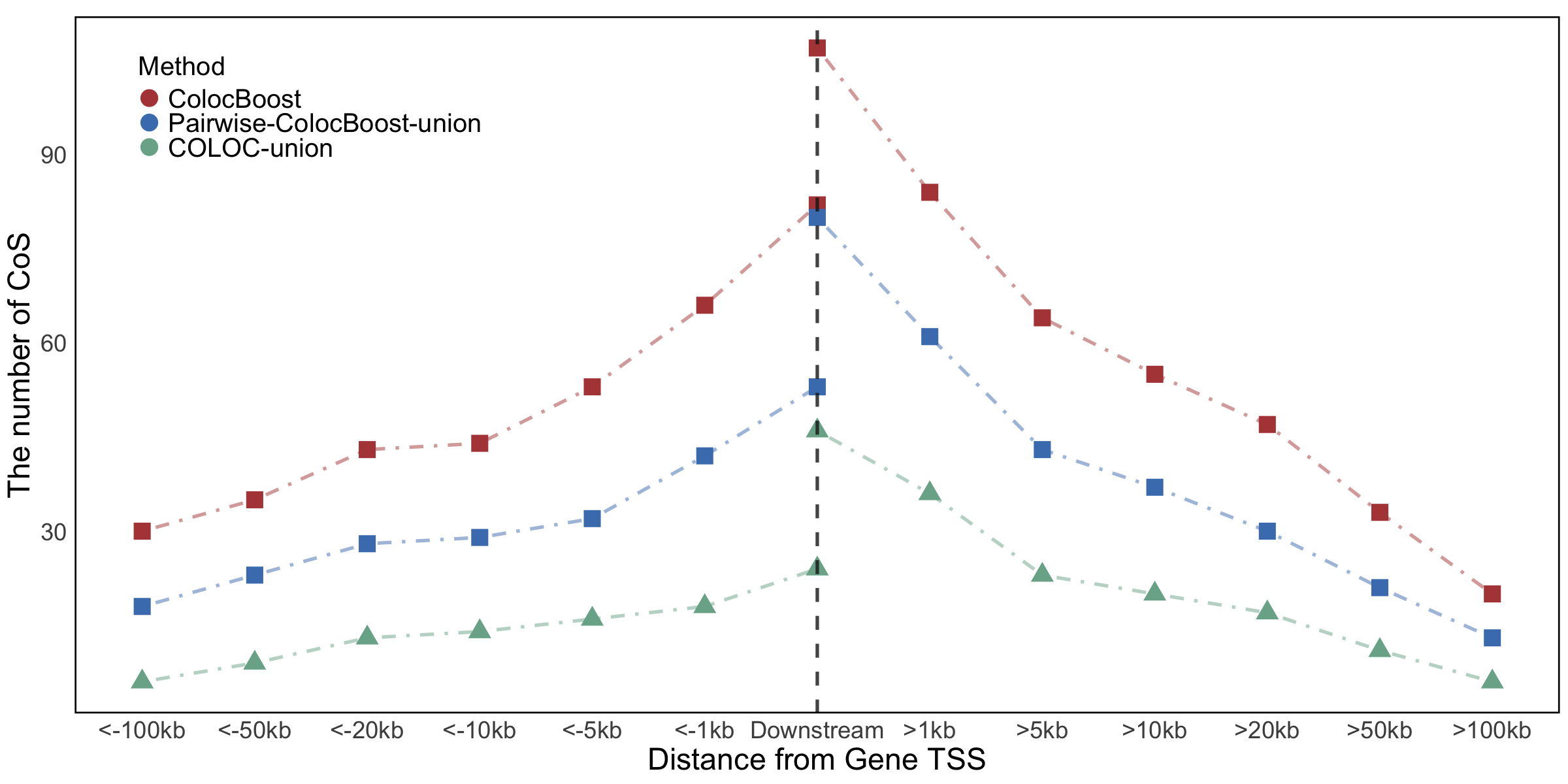
Figure 6c. Distribution of distances from the gene TSS for CoS.

Distribution of distances from the gene TSS for CoS from AD–xQTL ColocBoost, COLOC-union, and the union of CoS identified by ColocBoost applied pairwise to one AD GWAS and each of xQTL traits (pairwise-ColocBoost-union).

data <- readRDS("Figure_6c.rds")
library(ggplot2)
p1 <- ggplot(data, aes(x = Dist, y = cumsum_count, color = group, shape = group)) +
  geom_point(size = 7) +
  geom_line(data = subset(data, cate == "Upstream"), aes(group = group), linewidth = 1.5, alpha = 0.5, linetype = 4) + 
  geom_line(data = subset(data, cate == "Downstream"), aes(group = group), linewidth = 1.5, alpha = 0.5, linetype = 4) + 
  geom_vline(xintercept = 7, color = "grey10", linetype = 2, linewidth = 1.5, alpha = 0.8) +
  scale_shape_manual(values = c("COLOC-union" = 17, "ColocBoost" = 15, "Pairwise-ColocBoost-union" = 15)) + 
  guides(shape = "none") +
  scale_color_manual(values = c("COLOC-union" = "#79AF97FF", 
                                "Pairwise-ColocBoost-union" = "#4A7EBBFF",
                                "ColocBoost" = "#B24745FF")) +
  theme_minimal(base_size = 15) +
  labs(
    title = "",
    x = "Distance from Gene TSS",
    y = "The number of CoS",
    color = "Method",
    shape = "Category"
  ) +
  theme(
    plot.title = element_text(size = 0),
    axis.title.x = element_text(size = 28),
    axis.title.y = element_text(size = 28),
    axis.text.x = element_text(size = 22), #, angle = 30, vjust = 0.5, hjust = 0.5),
    axis.text.y = element_text(size = 22),
    legend.title = element_text(size = 24),
    legend.text = element_text(size = 24),
    legend.position = "inside",
    strip.text = element_text(size = 0, face = "bold"),
    legend.justification = c(0.05, 0.95),
    panel.grid.major = element_blank(),
    panel.grid.minor = element_blank(),
    panel.border = element_rect(color = "black", fill = NA, linewidth = 1.5)
  )

options(repr.plot.width = 20, repr.plot.height = 10)
p1