Figure S3. Additional metrics to benchmark performance of ColocBoost with other multi-trait colocalization methods.

Figure S3. Additional metrics to benchmark performance of ColocBoost with other multi-trait colocalization methods.#

S3a. Statistical power and FDR of all methods based on the single top-ranked variant, involving 2, 5,10, and 20 phenotypes with up to five true causal variants, with genotype data and induced colocalization configurations designed to mimic real xQTL datasets (Methods).
S3b.Statistical power and FDR comparison of ColocBoost and OPERA for GWAS targeted colocalization, evaluated at the gene level, under the same simulation design used in OPERA.
S3c. Statistical power and FDR comparison and S3d variant-level precision-recall curves by varying the colocalization score threshold in a simulation design incorporating trait-trait correlations across 2, 5,10, and 20 phenotypes with up to five true causal variants.
S3e. Statistical power and FDR of ColocBoost and HyPrColoc assuming diagonal LD matrix and imposing a single-causal-variant assumption without LD-proximity smoothing in ColocBoost.
S3f. Statistical power and FDR for single trait fine-mapping analysis (FineBoost) with up to five causal variants using SuSiE and FineBoost (the single-trait version of ColocBoost) in simulation scenarios comprising up to five causal variants.

The error bars in panels b-g represent 95% confidence intervals.

Figure S3a#

Statistical power and FDR of all methods based on the single top-ranked variant, involving 2, 5,10, and 20 phenotypes with up to five true causal variants, with genotype data and induced colocalization configurations designed to mimic real xQTL datasets (Methods).

library(ggplot2)
library(ggpattern)
library(ggpubr)
library(cowplot)
sumstat = readRDS("Figure_S3a.rds")
colors_man <- c("#B24745FF", "#00A1D5FF", "#79AF97FF", "#DF8F44FF")
p1 <- sumstat %>% 
  ggplot(aes(x = as.character(max_causal), y = power, fill = method)) +
  geom_col(position = "dodge", width = 0.7, colour = "grey20", alpha = 0.8) +
  theme_minimal() + 
  ylim(0, 1.05) + 
  #scale_x_continuous(breaks = 1:max(sumstat$total_causal_var_number)) +  # Ensures x-axis ticks are integers
  facet_wrap(.~ marginal_trait_number,
             labeller = labeller(marginal_trait_number = function(x) paste("Number of Traits:", x)), scales = "free_x", nrow = 1) +
  geom_errorbar(aes(ymin = power - 1.96*power_SD/ sqrt(20) , 
                    ymax = power + 1.96*power_SD/ sqrt(20) ),
                width = .2, position = position_dodge(width = 0.7)) +
  scale_fill_manual(values = colors_man, name = "Methods") +
  # guides(fill = guide_legend(title = "Methods")) + 
  labs(x = "Max Number of True Causal Variants Per Trait", y = "Power", color = "Methods") +
  theme(legend.position = "none",
        axis.title.x = element_text(size = 24), 
        axis.title.y = element_text(size = 30),
        axis.text.x = element_text(size = 22), 
        axis.text.y = element_text(size = 22),
        strip.text = element_text(size = 16, face = "bold"),
        legend.title = element_text(size = 24, face = "bold", margin = margin(l = 0, r= 20)),  # Change legend title font size and style
        legend.text = element_text(size = 24, margin = margin(l = 5, r= 8)),
        text=element_text(size=24,  family="sans")) + theme(
          panel.grid.major = element_blank(),      # Remove major grid lines
          panel.grid.minor = element_blank(),      # Remove minor grid lines
          #     axis.line = element_line(color = "black") # Keep the axis lines
        )

p2 <- sumstat %>% 
  ggplot(aes(x = as.character(max_causal), y = FDR, fill = method)) +
  geom_col(position = "dodge", width = 0.7, colour = "grey20", alpha = 0.8) +
  theme_minimal() + 
  ylim(0, 1) +
  #scale_x_continuous(breaks = 1:max(sumstat$total_causal_var_number)) +  # Ensures x-axis ticks are integers
  facet_wrap(.~ marginal_trait_number,
             labeller = labeller(marginal_trait_number = function(x) paste("Number of Traits:", x)), scales = "free_x", nrow = 1) +
  geom_errorbar(aes(ymin = FDR - 1.96 * FDR_SD / sqrt(20), 
                    ymax = FDR + 1.96 *FDR_SD / sqrt(20)),
                width = .2, position = position_dodge(width = 0.7)) +
  scale_fill_manual(values = colors_man, name = "Methods") +
  # guides(fill = guide_legend(title = "Methods")) + 
  labs(x = "Max Number of True Causal Variants Per Trait", y = "FDR", color = "Methods") +
  geom_hline(yintercept = 0.05, linetype = "dashed", color = "red", linewidth = 0.6) +
  # geom_hline(yintercept = 0.1, linetype = "dashed", color = "blue", linewidth = 0.6) +
  theme(legend.position = "bottom",
        axis.title.x = element_text(size = 24), 
        axis.title.y = element_text(size = 30),
        axis.text.x = element_text(size = 22), 
        axis.text.y = element_text(size = 22),
        strip.text = element_text(size = 16, face = "bold"),
        legend.title = element_text(size = 24, face = "bold", margin = margin(l = 0, r= 20)),  # Change legend title font size and style
        legend.text = element_text(size = 24, margin = margin(l = 5, r= 8)),
        text=element_text(size=24,  family="sans")) + theme(
          panel.grid.major = element_blank(),      # Remove major grid lines
          panel.grid.minor = element_blank(),      # Remove minor grid lines
          # axis.line = element_line(color = "black") # Keep the axis lines
        )

options(repr.plot.width = 16, repr.plot.height = 10)
plot_grid(p1, p2, ncol = 1)

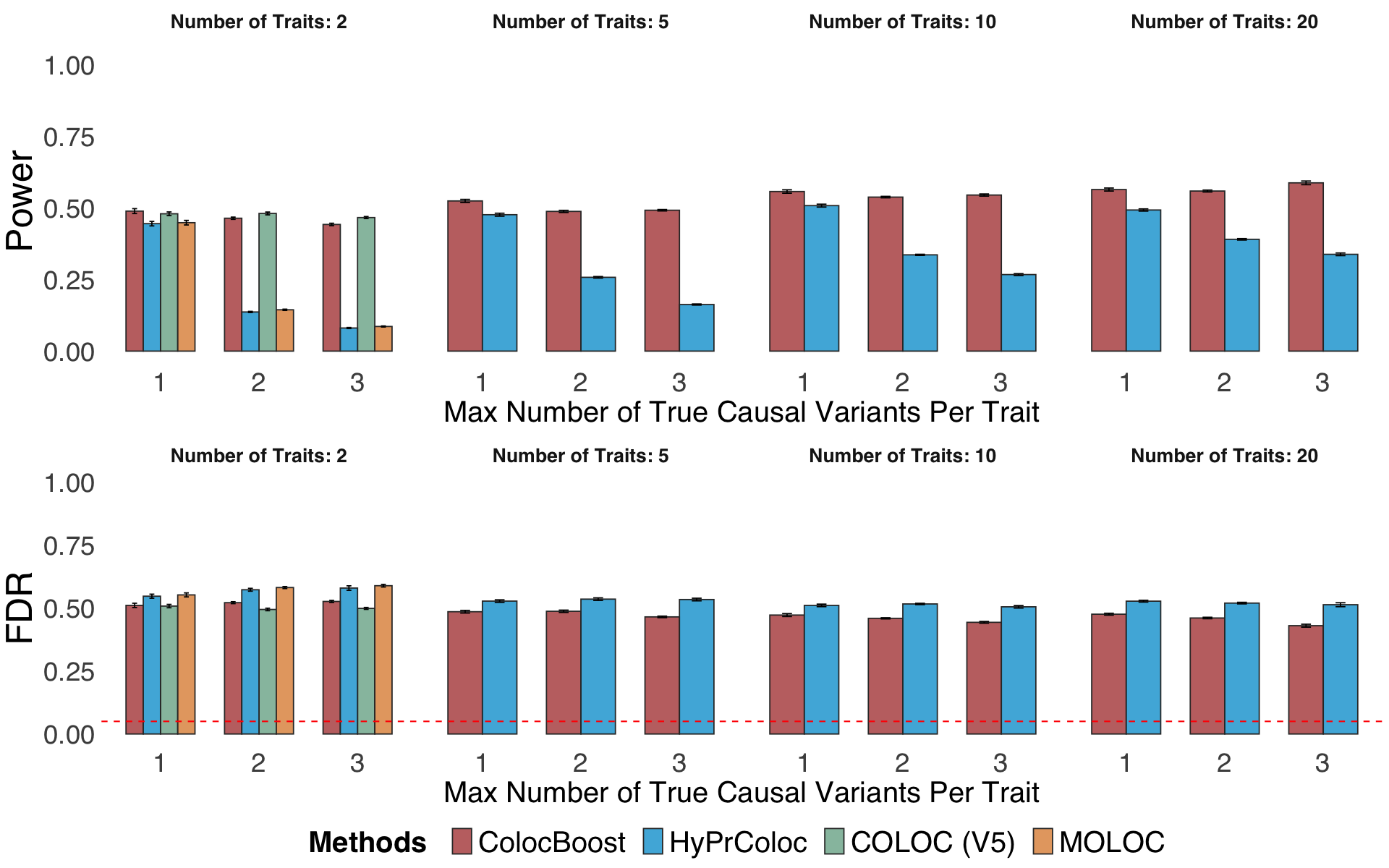
../../_images/423dafc6390f80946262190c896e2a6f6899458c11125b2942bf8908353accdd.png

Figure S3b#

Statistical power and FDR comparison of ColocBoost and OPERA for GWAS targeted colocalization, evaluated at the gene level, under the same simulation design used in OPERA.

library(ggplot2)
sumstat = readRDS("Figure_S3b.rds")
colors_man <- c("#B24745FF", "#1d4a9e")
p1 <- sumstat %>% 
  ggplot(aes(x = as.factor(trait), y = power, fill = method)) +
  #facet_wrap( ~ trait, labeller = labeller(trait = function(x) paste("Number of Traits:", x)), scales = "free_x", nrow = 1) +
  geom_col(position = "dodge", width = 0.7, colour = "grey20", alpha = 0.8) +
  theme_minimal() + 
  ylim(0, 1.05)  +  # Ensures x-axis ticks are integers
  geom_errorbar(aes(ymin = power - 1.96*power_SD/ sqrt(20) , 
                    ymax = power + 1.96*power_SD/ sqrt(20) ),
                width = .2, position = position_dodge(width = 0.7)) +
  scale_fill_manual(values = colors_man, name = "Methods") +
  # guides(fill = guide_legend(title = "Methods")) + 
  labs(x = "Number of Traits", y = "Power", color = "Methods") +
  theme(legend.position = "none",
        axis.title.x = element_text(size = 0),
        axis.title.y = element_text(size = 26),
        axis.text.x = element_text(size = 20),
        axis.text.y = element_text(size = 20),
        strip.text = element_text(size = 24, face = "bold"),
        legend.title = element_text(size = 24, face = "bold", margin = margin(l = 0, r= 20)),  # Change legend title font size and style
        legend.text = element_text(size = 20, margin = margin(l = 5, r= 8)),
        text=element_text(size=16,  family="sans")) + theme(
          panel.grid.major = element_blank(),      # Remove major grid lines
          panel.grid.minor = element_blank(),      # Remove minor grid lines
          # axis.line = element_line(color = "black") # Keep the axis lines
        )

p2 <- sumstat %>% 
  ggplot(aes(x = as.factor(trait), y = FDR, fill = method)) +
  geom_col(position = "dodge", width = 0.7, colour = "grey20", alpha = 0.8) +
  theme_minimal() + 
  #facet_wrap( ~ trait, labeller = labeller(trait = function(x) paste("Number of Traits:", x)), scales = "free_x", nrow = 1) +
  ylim(0, 0.2) +  # Ensures x-axis ticks are integers
  geom_errorbar(aes(ymin = FDR - 1.96 * FDR_SD / sqrt(20), 
                    ymax = FDR + 1.96 *FDR_SD / sqrt(20)),
                width = .2, position = position_dodge(width = 0.7)) +
  scale_fill_manual(values = colors_man, name = "Methods") +
  labs(x = "Number of Traits", y = "FDR", color = "Methods") +
  geom_hline(yintercept = 0.05, linetype = "dashed", color = "red", linewidth = 0.6) +
  theme(legend.position = "inside",
        axis.title.x = element_text(size = 24),
        axis.title.y = element_text(size = 26),
        axis.text.x = element_text(size = 20),
        axis.text.y = element_text(size = 20),
        strip.text = element_text(size = 24, face = "bold"),
        legend.title = element_text(size = 24, face = "bold", margin = margin(l = 0, r= 20)),  # Change legend title font size and style
        legend.text = element_text(size = 20, margin = margin(l = 5, r= 8)),
        text=element_text(size=16,  family="sans")) + theme(
          panel.grid.major = element_blank(),      # Remove major grid lines
          panel.grid.minor = element_blank(),      # Remove minor grid lines
          # axis.line = element_line(color = "black") # Keep the axis lines
        )

options(repr.plot.width = 6, repr.plot.height = 10)
plot_grid(p1, p2, ncol = 1)

../../_images/0b4084c2d26920450343ff7a38d6e41eedb6d22cd0597d2ec0dfa374d1710422.png

Figure S3c#

Statistical power and FDR comparison by varying the colocalization score threshold in a simulation design incorporating trait-trait correlations across 2, 5,10, and 20 phenotypes with up to five true causal variants.

library(ggplot2)
library(ggpattern)
library(ggpubr)
library(cowplot)
sumstat = readRDS("Figure_S3c.rds")
colors_man <- c("#B24745FF", "#00A1D5FF", "#79AF97FF", "#DF8F44FF")
p1 <- sumstat %>% 
  ggplot(aes(x = as.character(max_causal), y = power, fill = method)) +
  geom_col(position = "dodge", width = 0.7, colour = "grey20", alpha = 0.8) +
  theme_minimal() + 
  ylim(0, 1.05)  +  # Ensures x-axis ticks are integers
  geom_errorbar(aes(ymin = power - 1.96*power_SD/ sqrt(20) , 
                    ymax = power + 1.96*power_SD/ sqrt(20) ),
                width = .2, position = position_dodge(width = 0.7)) +
  scale_fill_manual(values = colors_man, name = "Methods") +
  facet_wrap(.~ marginal_trait_number,
             labeller = labeller(marginal_trait_number = function(x) paste("Number of Traits:", x)), scales = "free_x", nrow = 1) +
  labs(x = "Simulation Design", y = "Power", color = "Methods", title = NULL) +
  theme(legend.position = "none",
        plot.title = element_text(size = 26, face = "bold", hjust = 0.5),
        axis.title.x = element_text(size = 0),
        axis.title.y = element_text(size = 26),
        axis.text.x = element_text(size = 20),
        axis.text.y = element_text(size = 20),
        strip.text = element_text(size = 24, face = "bold"),
        legend.title = element_text(size = 24, face = "bold", margin = margin(l = 0, r= 20)),  # Change legend title font size and style
        legend.text = element_text(size = 20, margin = margin(l = 5, r= 8)),
        text=element_text(size=16,  family="sans")) + theme(
          panel.grid.major = element_blank(),      # Remove major grid lines
          panel.grid.minor = element_blank(),      # Remove minor grid lines
          # axis.line = element_line(color = "black") # Keep the axis lines
        )

p2 <- sumstat %>% 
  ggplot(aes(x = as.character(max_causal), y = FDR, fill = method)) +
  geom_col(position = "dodge", width = 0.7, colour = "grey20", alpha = 0.8) +
  theme_minimal() + 
  ylim(0, 0.2) +  # Ensures x-axis ticks are integers
  geom_errorbar(aes(ymin = FDR - 1.96*sqrt(FDR * (1-FDR)/total_trait_number), 
                    ymax = FDR + 1.96*sqrt(FDR * (1-FDR)/total_trait_number)),
                width = .2, position = position_dodge(width = 0.7)) +
  scale_fill_manual(values = colors_man, name = "Methods") +
  facet_wrap(.~ marginal_trait_number,
             labeller = labeller(marginal_trait_number = function(x) paste("Number of Traits:", x)), scales = "free_x", nrow = 1) +
  labs(x = "Simulation Design", y = "FDR", color = "Methods") +
  geom_hline(yintercept = 0.05, linetype = "dashed", color = "red", linewidth = 0.6) +
  labs(x = "Max Number of True Causal Variants Per Trait", y = "FDR", color = "Methods") +
  #geom_hline(yintercept = 0.1, linetype = "dashed", color = "blue", linewidth = 0.6) +
  theme(legend.position = "inside",
        axis.title.x = element_text(size = 26),
        axis.title.y = element_text(size = 26),
        axis.text.x = element_text(size = 20),
        axis.text.y = element_text(size = 20),
        strip.text = element_text(size = 24, face = "bold"),
        legend.title = element_text(size = 24, face = "bold", margin = margin(l = 0, r= 20)),  # Change legend title font size and style
        legend.text = element_text(size = 20, margin = margin(l = 5, r= 8)),
        legend.justification = c(0, 0.9),
        text=element_text(size=16,  family="sans")) + theme(
          panel.grid.major = element_blank(),      # Remove major grid lines
          panel.grid.minor = element_blank(),      # Remove minor grid lines
          # axis.line = element_line(color = "black") # Keep the axis lines
        )

options(repr.plot.width = 16, repr.plot.height = 10)
plot_grid(p1, p2, ncol = 1)

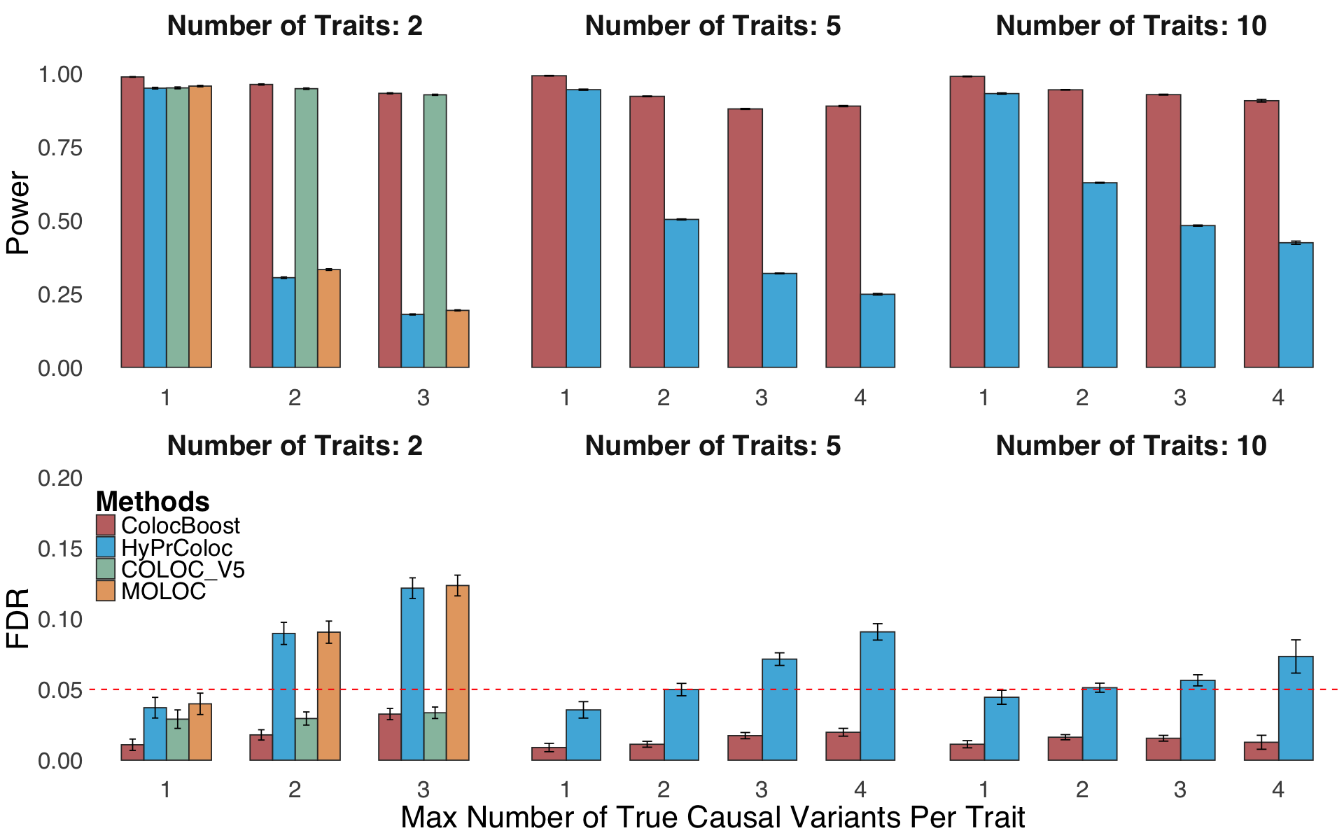
../../_images/eec85bb028594ae8f15c439f9e689aa303160ba2ae00bceaa14d3edba57db4c9.png

Figure S3d#

Variant-level precision-recall curves by varying the colocalization score threshold in a simulation design incorporating trait-trait correlations across 2, 5,10, and 20 phenotypes with up to five true causal variants.

library(ggplot2)
library(tidyverse)
all_dat = readRDS("Figure_S3d.rds")
colors_man <- c("#EE8E8F", "#87CEFA", "#98B892", "#E69B61")
p = all_dat %>%
  ggplot(aes(x = recall, y = mean, color = method)) +
  # Plot points where label == 1
  geom_point(data = filter(all_dat, label == 1), aes(x = recall, y = mean, color = method), 
             size = 5, shape = 16) +
  geom_line(linewidth= 0.5) + 
  geom_errorbar(aes(ymin = mean - 1.96 * se, 
                    ymax = mean + 1.96 * se), alpha = 0.4) +
  #scale_x_continuous(breaks = 1:max(sumstat$total_causal_var_number)) +  # Ensures x-axis ticks are integers
  facet_wrap(.~ trait,
             labeller = labeller(trait = function(x) paste("Number of Traits:", x)), scales = "free_x", nrow = 1) + 
  labs(x = "Variant-level Recall", y = "Variant-level Precision", color = "Methods")+
  theme_minimal()  +
  scale_color_manual(values = colors_man, name = "Methods")+
  theme(legend.position = "bottom",
        axis.title.x = element_text(margin = margin(t = 10), size = 20), 
        axis.title.y = element_text(size = 20),
        axis.text.x = element_text(size = 14), 
        axis.text.y = element_text(size = 14),
        strip.text = element_text(size = 16, face = "bold"),
        legend.title = element_text(size = 16, face = "bold", margin = margin(l = 0, r= 20)),  # Change legend title font size and style
        legend.text = element_text(size = 16, margin = margin(l = 5, r= 8)),
        text=element_text(size=16,  family="sans")) + theme(
          panel.grid.major = element_blank(),      # Remove major grid lines
          panel.grid.minor = element_blank(),      # Remove minor grid lines
          #axis.line = element_line(color = "black") # Keep the axis lines
        )

options(repr.plot.width = 16, repr.plot.height = 6)
p

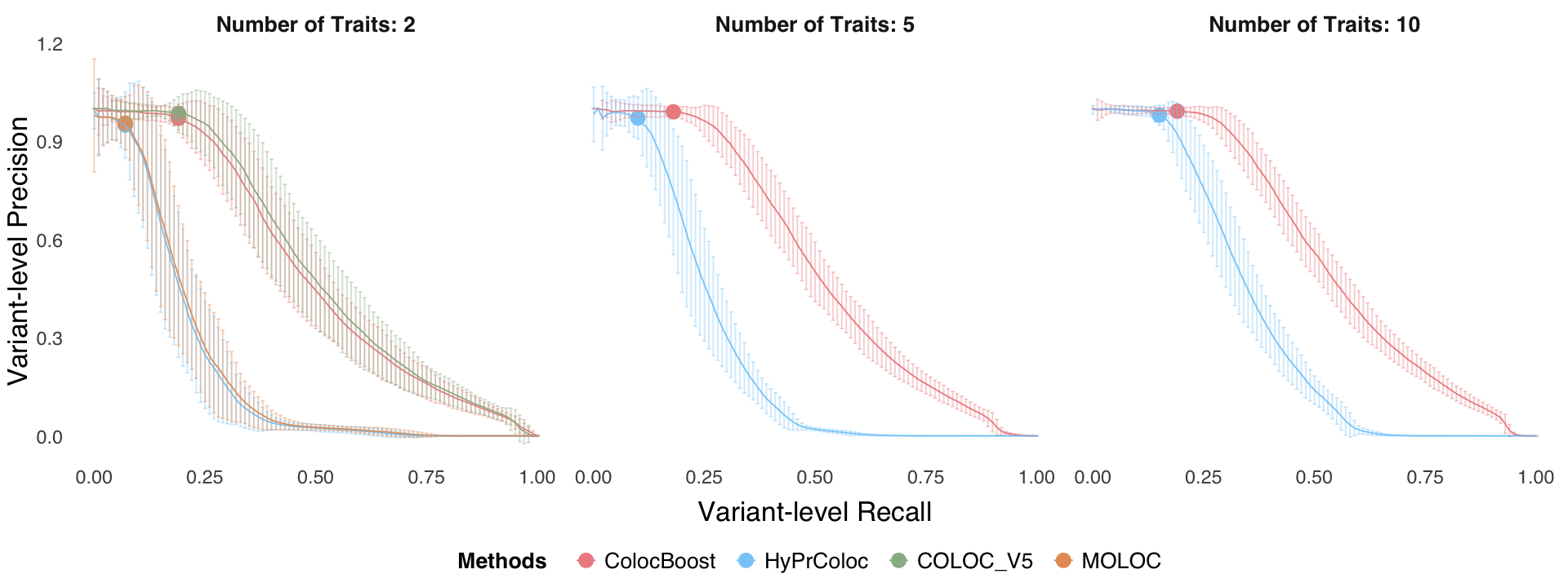
../../_images/f8198fe796b957b54c8507eee2c376a5d2442c5c6f7982333d2d4416b1a4a430.png

Figure S3e#

Statistical power and FDR of ColocBoost and HyPrColoc assuming diagonal LD matrix and imposing a single-causal-variant assumption without LD-proximity smoothing in ColocBoost.

library(ggplot2)
sumstat = readRDS("Figure_S3e.rds")
colors_man <- c("#B24745FF", "#00A1D5FF")
p1 <- sumstat %>% 
  ggplot(aes(x = as.character(causal_number), y = power, fill = method)) +
  geom_col(position = "dodge", width = 0.7, colour = "grey20") +
  theme_minimal() + 
  ylim(0, 1.05)  +  # Ensures x-axis ticks are integers
  geom_errorbar(aes(ymin = power - 1.96*sqrt(power * (1-power)/total_trait_number), 
                    ymax = power + 1.96*sqrt(power * (1-power)/total_trait_number)),
                width = .2, position = position_dodge(width = 0.7)) +
  scale_fill_manual(values = colors_man, name = "Methods") +
  facet_wrap(.~ trait_number,
             labeller = labeller(trait_number = function(x) paste("Number of Traits:", x)), scales = "free_x", nrow = 1) +
  # guides(fill = guide_legend(title = "Methods")) + 
  labs(x = "Simulation Design", y = "Power", color = "Methods") +
  theme(legend.position = "none",
        plot.title = element_text(size = 26, face = "bold", hjust = 0.5),
        axis.title.x = element_text(size = 0),
        axis.title.y = element_text(size = 26),
        axis.text.x = element_text(size = 0),
        axis.text.y = element_text(size = 20),
        strip.text = element_text(size = 24, face = "bold"),
        legend.title = element_text(size = 24, face = "bold", margin = margin(l = 0, r= 20)),  # Change legend title font size and style
        legend.text = element_text(size = 20, margin = margin(l = 5, r= 8)),
        text=element_text(size=16,  family="sans")) + theme(
          panel.grid.major = element_blank(),      # Remove major grid lines
          panel.grid.minor = element_blank(),      # Remove minor grid lines
          # axis.line = element_line(color = "black") # Keep the axis lines
        )

p2 <- sumstat %>% 
  ggplot(aes(x = as.character(causal_number), y = FDR, fill = method)) +
  geom_col(position = "dodge", width = 0.7, colour = "grey20") +
  theme_minimal() + 
  ylim(0, 0.2) +  # Ensures x-axis ticks are integers
  geom_errorbar(aes(ymin = FDR - 1.96*sqrt(FDR * (1-FDR)/total_trait_number), 
                    ymax = FDR + 1.96*sqrt(FDR * (1-FDR)/total_trait_number)),
                width = .2, position = position_dodge(width = 0.7)) +
  scale_fill_manual(values = colors_man, name = "Methods") +
  facet_wrap(.~ trait_number,
             labeller = labeller(trait_number = function(x) paste("Number of Traits:", x)), scales = "free_x", nrow = 1) +
  # guides(fill = guide_legend(title = "Methods")) + 
  labs(x = "Simulation Design", y = "FDR", color = "Methods") +
  geom_hline(yintercept = 0.05, linetype = "dashed", color = "red", linewidth = 0.6) +
  #geom_hline(yintercept = 0.1, linetype = "dashed", color = "blue", linewidth = 0.6) +
  theme(legend.position = "inside",
        axis.title.x = element_text(size = 0),
        axis.title.y = element_text(size = 26),
        axis.text.x = element_text(size = 20),
        axis.text.y = element_text(size = 20),
        strip.text = element_text(size = 24, face = "bold"),
        legend.title = element_text(size = 24, face = "bold", margin = margin(l = 0, r= 20)),  # Change legend title font size and style
        legend.text = element_text(size = 20, margin = margin(l = 5, r= 8)),
        text=element_text(size=16,  family="sans")) + theme(
          panel.grid.major = element_blank(),      # Remove major grid lines
          panel.grid.minor = element_blank(),      # Remove minor grid lines
          # axis.line = element_line(color = "black") # Keep the axis lines
      )

options(repr.plot.width = 16, repr.plot.height = 12)
plot_grid(p1, p2, ncol = 1)

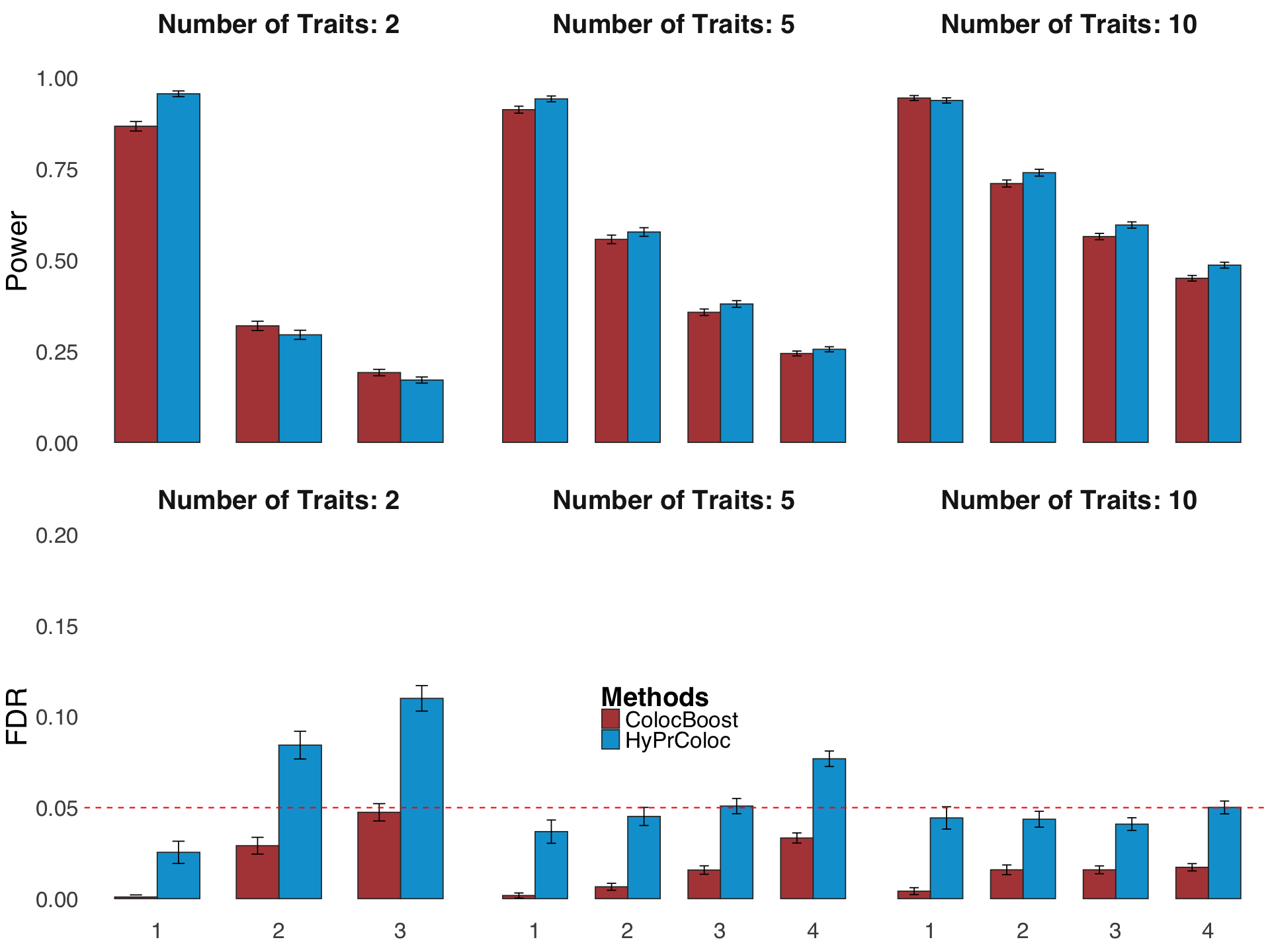
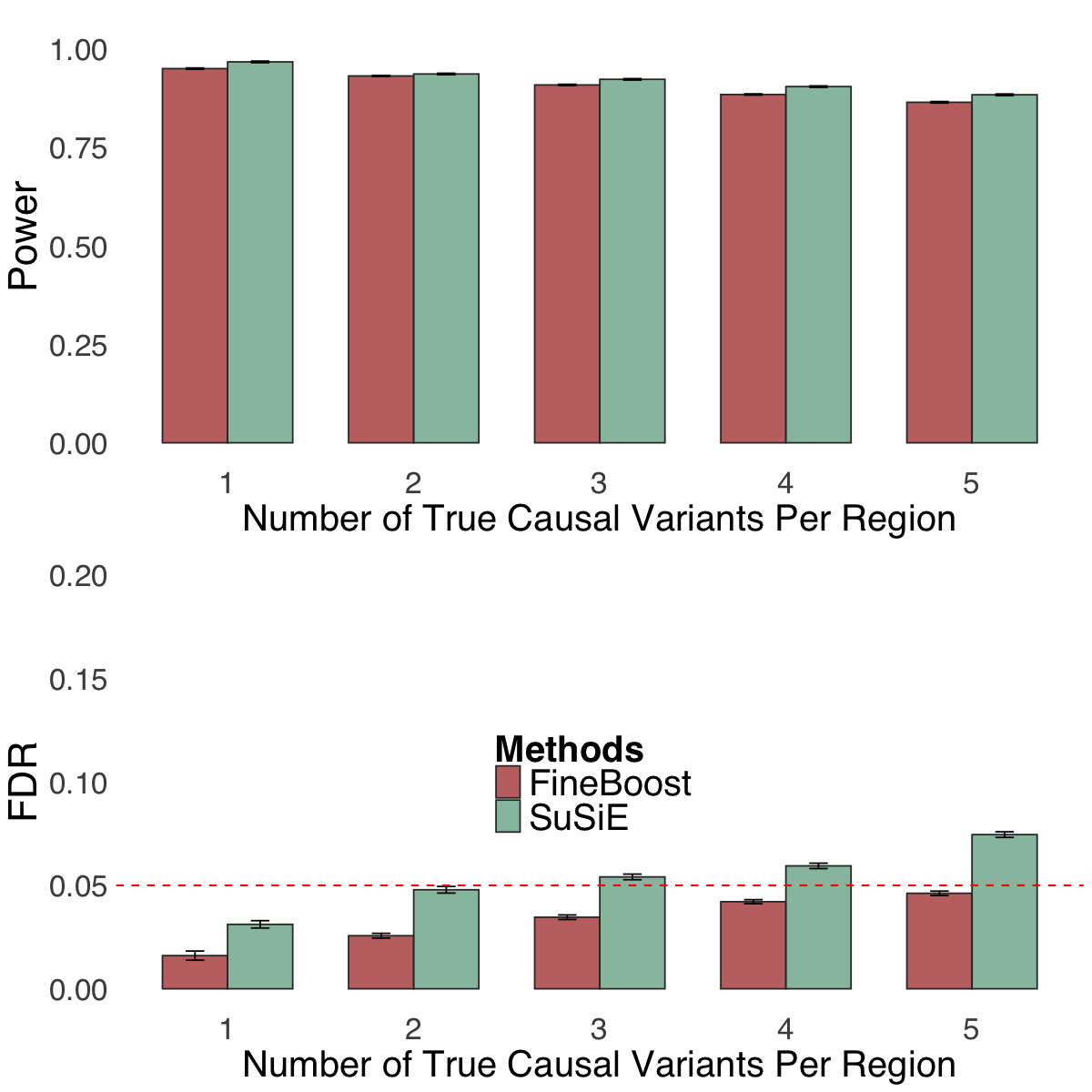
../../_images/a8f369da80056f25a89e47faa166deca807b442e983010c092d9db56927cd9ba.png

Figure S3f#

Statistical power and FDR for single trait fine-mapping analysis (FineBoost) with up to five causal variants using SuSiE and FineBoost (the single-trait version of ColocBoost) in simulation scenarios comprising up to five causal variants.

library(ggplot2)
sum_tb = readRDS("Figure_S3f.rds")
colors_man <- c("#B24745FF", "#79AF97FF")
p1 <- sum_tb %>% 
  ggplot(aes(x = as.factor(total_variant_number), y = power, fill = method)) +
  geom_col(position = "dodge", width = 0.7, colour = "grey20", alpha = 0.8) +
  theme_minimal() + 
  ylim(0, 1.05) +
  scale_fill_manual(values = colors_man, name = "Methods") +
  geom_errorbar(aes(ymin = power - 1.96*power_SD/ sqrt(20) , 
                    ymax = power + 1.96*power_SD/ sqrt(20) ),
                width = .2, position = position_dodge(width = 0.7)) +
  # guides(fill = guide_legend(title = "Methods")) + 
  labs(x = "Number of True Causal Variants Per Region", y = "Power", color = "Methods") +
  theme(legend.position = "none",
        axis.title.x = element_text(size = 24),
        axis.title.y = element_text(size = 26),
        axis.text.x = element_text(size = 20),
        axis.text.y = element_text(size = 20),
        strip.text = element_text(size = 24, face = "bold"),
        legend.title = element_text(size = 24, face = "bold", margin = margin(l = 0, r= 20)),  # Change legend title font size and style
        legend.text = element_text(size = 24, margin = margin(l = 5, r= 8)),
        text=element_text(size=16,  family="sans")) + theme(
          panel.grid.major = element_blank(),      # Remove major grid lines
          panel.grid.minor = element_blank(),      # Remove minor grid lines
          # axis.line = element_line(color = "black") # Keep the axis lines
        )

p2 <- sum_tb %>% 
  ggplot(aes(x = as.factor(total_variant_number), y = FDR, fill = method)) +
  geom_col(position = "dodge", width = 0.7, colour = "grey20", alpha = 0.8) +
  theme_minimal() + 
  ylim(0, 0.2) +
  #scale_x_continuous(breaks = 1:max(sumstat$total_causal_var_number)) +  # Ensures x-axis ticks are integers
  #geom_errorbar(aes(ymin = FDR - 1.96 * FDR_SD / sqrt(20), 
  #                 ymax = FDR + 1.96 *FDR_SD / sqrt(20)),
  #            width = .2, position = position_dodge(width = 0.7)) +
  scale_fill_manual(values = colors_man, name = "Methods") +
  # guides(fill = guide_legend(title = "Methods")) + 
  labs(x = "Number of True Causal Variants Per Region", y = "FDR", color = "Methods") +
  geom_errorbar(aes(ymin = FDR - 1.96 * FDR_SD / sqrt(20), 
                    ymax = FDR + 1.96 *FDR_SD / sqrt(20)),
                width = .2, position = position_dodge(width = 0.7)) +
  geom_hline(yintercept = 0.05, linetype = "dashed", color = "red", linewidth = 0.6) +
  # geom_hline(yintercept = 0.1, linetype = "dashed", color = "blue", linewidth = 0.6) +
  theme(legend.position = "inside",
        axis.title.x = element_text(size = 24),
        axis.title.y = element_text(size = 26),
        axis.text.x = element_text(size = 20),
        axis.text.y = element_text(size = 20),
        strip.text = element_text(size = 24, face = "bold"),
        legend.title = element_text(size = 24, face = "bold", margin = margin(l = 0, r= 20)),  # Change legend title font size and style
        legend.text = element_text(size = 24, margin = margin(l = 5, r= 8)),
        text=element_text(size=16,  family="sans")) + theme(
          panel.grid.major = element_blank(),      # Remove major grid lines
          panel.grid.minor = element_blank(),      # Remove minor grid lines
          # axis.line = element_line(color = "black") # Keep the axis lines
        )

options(repr.plot.width = 10, repr.plot.height = 10)
plot_grid(p1, p2, ncol = 1)

../../_images/ed12cd00609d5d5d0f011a1bb3c9841e40a9404973c29661c12b75b896da7a14.png