Proportion of Variance Explained and Heritability#
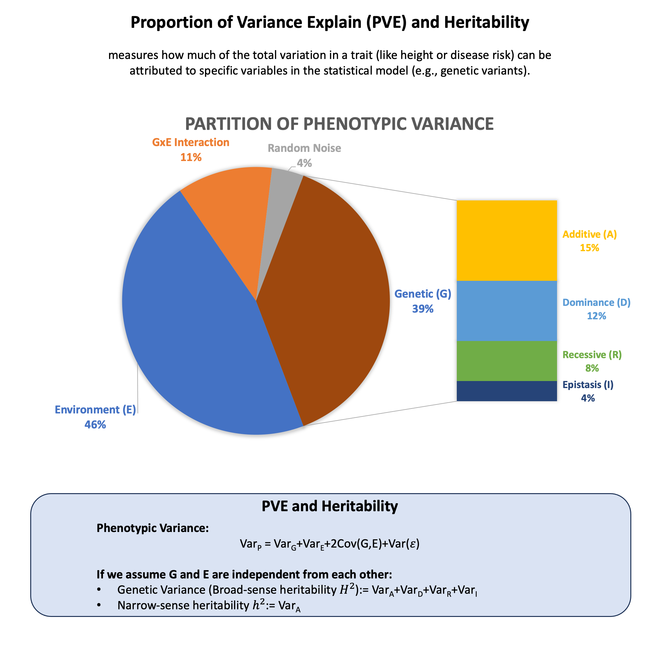
Proportion of variance explained (PVE) measures how much of the total variation in a trait (like height or disease risk) can be attributed to specific variables in your statistical model (e.g., genetic variants). Heritability is a specific application of this concept that measures how much of the variation in a trait across a population can be explained by genetic differences.
Graphical Summary#
Key Formula#
Any phenotype can be modeled as the sum of genetic (G) and environmental (E) effects, their interaction (G×E), and a residual error term (ε) that captures unexplained variation: \(Y = G + E + G \times E + \epsilon\). Under the assumptions that (1) genetic and environmental effects are independent, i.e., \(\text{Cov}(G,E) = 0\), and (2) the error term is uncorrelated with genetic effects, i.e., \(\text{Cov}(G,\epsilon) = 0\), the proportion of variance explained (PVE) by genetic effects alone (also called broad-sense heritability \(H^2\)) can be derived as:
where:
\(\sigma^2_G\) is the genetic variance component
\(\sigma^2_Y\) is the total phenotypic variance
Technical Details#
Generative Model#
A formal generative model specifies the probability distributions and relationships between variables:
where the components follow:
Key independence assumptions one can generally make:
\(G \perp E\) (genetic and environmental effects are independent)
\(G \perp \epsilon\) (genotype uncorrelated with residual error)
\(E \perp \epsilon\) (environment uncorrelated with residual error)
Violations occur when omitted confounders correlate with genotype, or when \(G \times E\) interactions exist but aren’t modeled, causing them to be absorbed into \(\epsilon\).
Variance Decomposition#
Under the independence assumptions:
If independence is violated (e.g., \(\text{Cov}(G,E) \neq 0\) or \(\text{Cov}(G,\epsilon) \neq 0\)), covariance terms appear:
This leads to biased heritability estimates. In practice, \(\sigma^2_E\) and \(\sigma^2_{\epsilon}\) are often combined since distinguishing environmental from residual variance requires experimental manipulation.
Broad-sense Heritability#
This represents the proportion of phenotypic variance from all genetic effects (additive + dominance + epistatic). \(H^2\) is population- and environment-specific, not a fixed biological constant.
Narrow-sense Heritability#
The genetic variance can be decomposed into:
where \(\sigma^2_A\) is additive variance, \(\sigma^2_D\) is dominance variance, \(\sigma^2_R\) is recessive variance, and \(\sigma^2_I\) is epistatic variance.
Narrow-sense heritability captures only additive genetic effects. This is what GWAS, eQTL mapping, and polygenic risk scores estimate, since these methods model linear allelic effects. The difference \(H^2 - h^2\) reflects non-additive genetic architecture.
Example#
When we say a trait has “50% heritability,” we mean 50% of the variation in that trait across individuals is due to genetic differences. Let’s explore this with 100 individuals whose phenotype is influenced by:
Variant 1: additive effect
Variant 2: dominant effect (any non-zero genotype)
Interaction between variants 1 and 2
Environmental factor
Residual/unexplained variation
We’ll calculate \(H^2\) (broad-sense heritability) and \(h^2\) (narrow-sense heritability) under both fixed and random effect models.
Setup#
rm(list = ls())
set.seed(11)

# Define parameters
N <- 100  # Number of individuals
M <- 2    # Number of variants

# Generate genotype data directly as allele counts (0, 1, 2)
# Variant 1: additive effect, MAF = 0.3
variant1 <- sample(0:2, N, replace = TRUE, prob = c(0.49, 0.42, 0.09))

# Variant 2: dominance effect, MAF = 0.5
variant2 <- sample(0:2, N, replace = TRUE, prob = c(0.25, 0.5, 0.25))

# Combine into raw genotype matrix
X_raw <- cbind(variant1, variant2)
rownames(X_raw) <- paste("Individual", 1:N)
colnames(X_raw) <- c("Variant1_Additive", "Variant2_Dominant")

# Create dominance coding for variant 2
# Dominance coding: 1 if genotype is not 0 (i.e., has at least one alternative allele)
Xraw_dominance <- ifelse(X_raw[, 2] != 0, 1, 0)

# Create interaction term: variant1 (additive) × variant2 (dominance)
Xraw_interaction <- X_raw[, 1] * Xraw_dominance

# Generate environmental variable
# For example, this could represent diet, exercise, stress, etc.
E_raw <- rnorm(N, mean = 0, sd = 1)

# Standardize all components
X_additive <- scale(X_raw[, 1], center = TRUE, scale = TRUE)
X_dominance <- scale(Xraw_dominance, center = TRUE, scale = TRUE)
X_interaction <- scale(Xraw_interaction, center = TRUE, scale = TRUE)
E <- scale(E_raw, center = TRUE, scale = TRUE)
Fixed Effect#
Effect sizes are constant parameters:
# Fixed effects: constant effect sizes
beta_A <- 0.8   # Additive effect
beta_D <- 0.6   # Dominance effect
beta_I <- 0.4   # Interaction effect
beta_E <- 0.5   # Environmental effect

# Generate phenotype
epsilon <- rnorm(N, mean = 0, sd = 1)
Y <- X_additive * beta_A + X_dominance * beta_D + X_interaction * beta_I + E * beta_E + epsilon
Calculate variance components and heritability:
# Calculate variance components
var_A <- var(X_additive * beta_A)
var_D <- var(X_dominance * beta_D)
var_I <- var(X_interaction * beta_I)
var_G <- var_A + var_D + var_I
var_E <- var(E * beta_E)
var_epsilon <- var(epsilon)
var_Y <- var(Y)
# Calculate heritabilities
H2 <- var_G / var_Y
h2 <- var_A / var_Y
# Display results
cat("Heritability:\n")
cat(" H² (broad-sense): ", round(H2, 4), "\n")
cat(" h² (narrow-sense): ", round(h2, 4), "\n")
cat(" H² - h² (non-additive):", round(H2 - h2, 4), "\n")
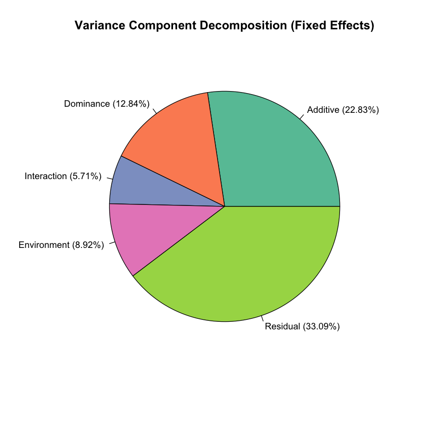
# Create pie chart of variance components
library(RColorBrewer)
colors <- brewer.pal(5, "Set2")
variance_data <- c(var_A, var_D, var_I, var_E, var_epsilon)
variance_labels <- c(
paste0("Additive (", round(var_A/var_Y*100, 2), "%)"),
paste0("Dominance (", round(var_D/var_Y*100, 2), "%)"),
paste0("Interaction (", round(var_I/var_Y*100, 2), "%)"),
paste0("Environment (", round(var_E/var_Y*100, 2), "%)"),
paste0("Residual (", round(var_epsilon/var_Y*100, 2), "%)")
)
pie(variance_data, labels = variance_labels, col = colors,
main = "Variance Component Decomposition (Fixed Effects)",
cex = 0.9)
Heritability:
  H² (broad-sense):       0.4138
  h² (narrow-sense):      0.2283
  H² - h² (non-additive): 0.1855
Random effect#
Effect sizes are drawn from distributions for each individual:
# Random effects: draw effect sizes from distributions
beta_A_random <- rnorm(N, mean = 0, sd = 1.0)
beta_D_random <- rnorm(N, mean = 0, sd = 0.8)
beta_I_random <- rnorm(N, mean = 0, sd = 0.5)
beta_E_random <- rnorm(N, mean = 0, sd = 0.6)
Generate phenotype and calculate heritability:
# Generate phenotype with random effects
epsilon <- rnorm(N, mean = 0, sd = 1)
Y <- X_additive * beta_A_random + X_dominance * beta_D_random + X_interaction * beta_I_random + E * beta_E_random + epsilon
# Calculate variance components
var_A_random <- var(X_additive * beta_A_random)
var_D_random <- var(X_dominance * beta_D_random)
var_I_random <- var(X_interaction * beta_I_random)
var_G_random <- var_A_random + var_D_random + var_I_random
var_E_random <- var(E * beta_E_random)
var_epsilon_random <- var(epsilon)
var_Y_random <- var(Y)
# Calculate heritabilities
H2_random <- var_G_random / var_Y_random
h2_random <- var_A_random / var_Y_random
# Display results
cat("Heritability (Random Effects):\n")
cat(" H² (broad-sense): ", round(H2_random, 4), "\n")
cat(" h² (narrow-sense): ", round(h2_random, 4), "\n")
cat(" H² - h² (non-additive):", round(H2_random - h2_random, 4), "\n")
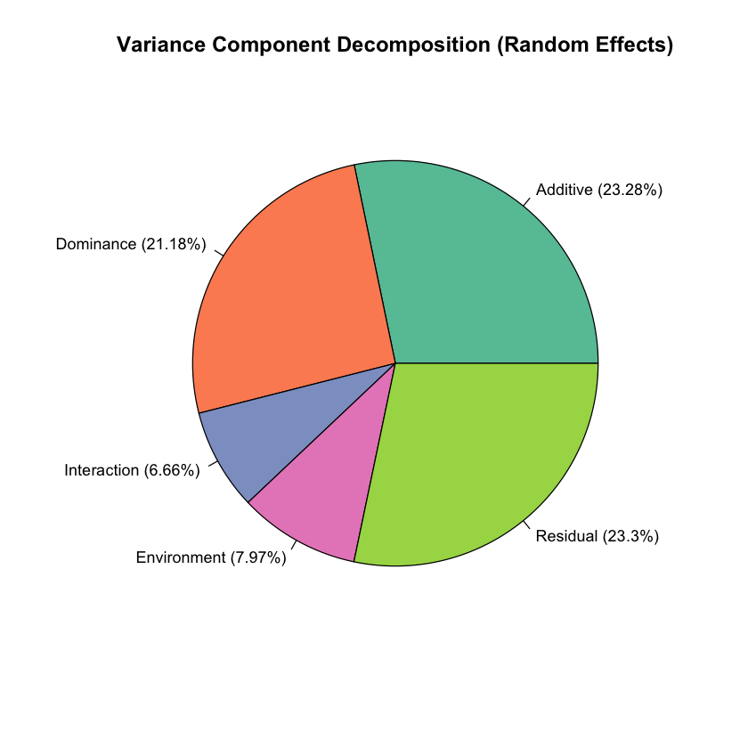
# Create pie chart of variance components
variance_data_random <- c(var_A_random, var_D_random, var_I_random, var_E_random, var_epsilon_random)
variance_labels_random <- c(
paste0("Additive (", round(var_A_random/var_Y_random*100, 2), "%)"),
paste0("Dominance (", round(var_D_random/var_Y_random*100, 2), "%)"),
paste0("Interaction (", round(var_I_random/var_Y_random*100, 2), "%)"),
paste0("Environment (", round(var_E_random/var_Y_random*100, 2), "%)"),
paste0("Residual (", round(var_epsilon_random/var_Y_random*100, 2), "%)")
)
pie(variance_data_random, labels = variance_labels_random, col = colors,
main = "Variance Component Decomposition (Random Effects)",
cex = 0.9)
Heritability (Random Effects):
  H² (broad-sense):       0.5112
  h² (narrow-sense):      0.2328
  H² - h² (non-additive): 0.2784