Ordinary Least Squares#
Single marker linear regression measures how well a genetic variant “aligns” with a trait by projecting the trait values onto the variant’s genotype direction.
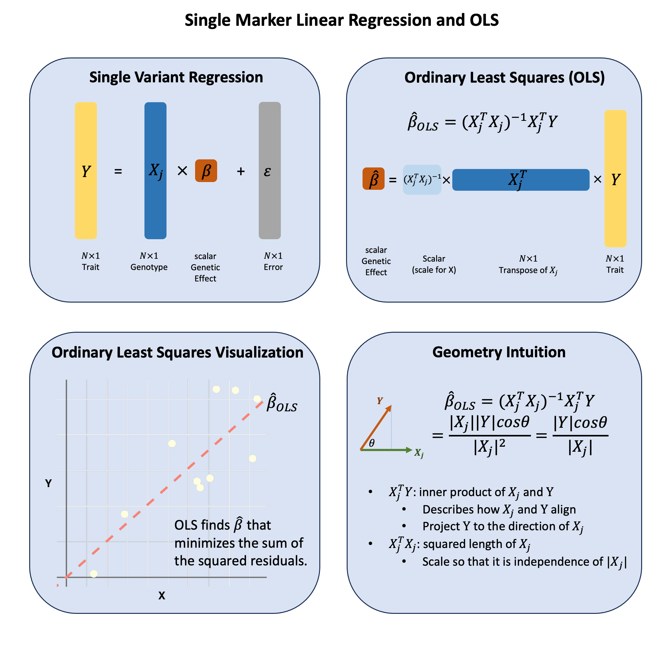
Graphical Summary#
Key Formula#
In the single marker linear regression
\(\mathbf{Y}\) is the \(N \times 1\) vector of trait values for \(N\) individuals
\(\mathbf{X}\) is the \(N \times 1\) vector of the genotype vector for a single variant across \(N\) individuals
\(\beta\) is the scalar representing the effect size for the variant (to be estimated)
\(\boldsymbol{\epsilon} \sim N(\mathbf{0}, \sigma^2)\) is the \(N \times 1\) vector of error terms for \(N\) individuals
Using ordinary least squares (OLS), we can derive the estimators for \(\beta\) as:
Technical Details#
Genomic Intuition#
The OLS estimator has a beautiful geometric interpretation that makes intuitive sense in genomics: OLS measures how much two vectors align in the same direction through their inner product, scaled by the variance of \(\mathbf{X}\).
The Inner Product \(\mathbf{X}^T\mathbf{Y}\): This measures the projection of the phenotype vector \(\mathbf{Y}\) onto the genotype vector \(\mathbf{X}\). In genomic terms, it captures how much the phenotype and genotype “move together” - when genotype values are high, are phenotype values also high? The inner product quantifies this concordance.
Why the Scaling Factor \((\mathbf{X}^T\mathbf{X})^{-1}\)?: This normalization is crucial because we want our measure of association to be scale-independent. Whether we code genotypes as (0,1,2) or (0,2,4), or measure height in centimeters versus meters, the strength of association shouldn’t change due to arbitrary scaling choices. The factor \((\mathbf{X}^T\mathbf{X})^{-1} = \frac{1}{\sum_{i=1}^N X_i^2}\) normalizes by the squared magnitude of the genotype vector, making the coefficient invariant to arbitrary scaling.
The Complete Picture: OLS finds the scalar that best aligns the genotype vector with the phenotype vector. It asks: “How much should I scale \(\mathbf{X}\) so it points as closely as possible toward \(\mathbf{Y}\)?” The answer is \(\hat{\beta}_\text{OLS}\).
Simplified Form for Single Marker Regression#
For a single marker regression, the OLS estimator simplifies to:
If genotypes are standardized (mean-centered and scaled to variance = 1), this becomes the sample covariance:
Unbiasedness#
Under the assumption that \(E[\epsilon|\mathbf{X}] = 0\):
The OLS estimator is unbiased for the true effect size.
Special Case: Centered Variables#
When both \(\mathbf{X}\) and \(\mathbf{Y}\) are mean-centered (\(\bar{X} = 0\), \(\bar{Y} = 0\)), the regression simplifies to regression through the origin.
Slope estimator: \(\hat{\beta}_{\text{OLS}} = \frac{\sum_{i=1}^N X_i Y_i}{\sum_{i=1}^N X_i^2}\)
Variance of the estimator: \(\text{Var}(\hat{\beta}_{\text{OLS}}) = \sigma^2 \cdot \frac{1}{\sum_{i=1}^N X_i^2} = \frac{\sigma^2}{\sum_{i=1}^N X_i^2}\)
Standard error: \(\text{SE}(\hat{\beta}_{\text{OLS}}) = \sqrt{\frac{\hat{\sigma}^2}{\sum_{i=1}^N X_i^2}}\)
where \(\hat{\sigma}^2 = \frac{\sum_{i=1}^N (Y_i - \hat{Y}_i)^2}{N-1}\) is the residual variance estimate. We use \(N-1\) degrees of freedom because we estimate only one parameter (the slope) when variables are centered.
Sample Size Requirements#
Absolute minimum: \(N \geq\) number of parameters to estimate
For regression through origin (centered case): \(N \geq 1\) technically, but \(N \geq 2\) for any practical inference
For regression with intercept: \(N \geq 2\)
Matrix \(\mathbf{X}^T\mathbf{X}\) must be invertible (full column rank required)
Larger \(N\) improves estimate precision and reduces uncertainty
In practice, for reliable inference, generally \(N \geq 30\) (rule of thumb)
Example#
In our toy example data of 5 individuals, now say we have also observed the height information for the 5 individuals. How do we actually perform OLS analysis to answer the question: do any of these variants actually influence height?
To begin with, we still converted those nucleotides into numbers as we did in Lecture: genotype coding, and after the transformation of the genotypes using an additive model, we apply our OLS formula both manually and using R’s built-in function. This will show you exactly how that geometric intuition - the projection and alignment between genotype and phenotype vectors - translates into real code and results.
Setup#
# Clear the environment
rm(list = ls())

# Define genotypes for 5 individuals at 3 variants
# These represent actual alleles at each position
# For example, Individual 1 has genotypes: CC, CT, AT
genotypes <- c(
 "CC", "CT", "AT",  # Individual 1
 "TT", "TT", "AA",  # Individual 2
 "CT", "CT", "AA",  # Individual 3
 "CC", "TT", "AA",  # Individual 4
 "CC", "CC", "TT"   # Individual 5
)
# Reshape into a matrix
N = 5
M = 3
geno_matrix <- matrix(genotypes, nrow = N, ncol = M, byrow = TRUE)
rownames(geno_matrix) <- paste("Individual", 1:N)
colnames(geno_matrix) <- paste("Variant", 1:M)

alt_alleles <- c("T", "C", "T")

# Convert to raw genotype matrix using the additive model
Xraw_additive <- matrix(0, nrow = N, ncol = M) # count number of non-reference alleles

rownames(Xraw_additive) <- rownames(geno_matrix)
colnames(Xraw_additive) <- colnames(geno_matrix)

for (i in 1:N) {
  for (j in 1:M) {
    alleles <- strsplit(geno_matrix[i,j], "")[[1]]
    Xraw_additive[i,j] <- sum(alleles == alt_alleles[j])
  }
}

X <- scale(Xraw_additive, center = TRUE, scale = TRUE)
We observe the heights (\(Y\)) for the five individuals as follows, and scale \(Y\) as well:
# assign observed height for the 5 individuals
Y_raw <- c(180, 160, 158, 155, 193)
Y <- scale(Y_raw)
OLS Regression#
We perform OLS analysis on each single SNP using lm function in R:
p_values <- numeric(M)  # Store p-values
betas <- numeric(M)     # Store estimated effect sizes

for (j in 1:M) {
  SNP <- X[, j]  # Extract genotype for SNP j
  model <- lm(Y ~ SNP)  # OLS regression: Trait ~ SNP
  summary_model <- summary(model)

  # Store p-value and effect size (coefficient)
  p_values[j] <- summary_model$coefficients[2, 4]  # p-value for SNP effect
  betas[j] <- summary_model$coefficients[2, 1]     # Estimated beta coefficient
}
The OLS results are:
OLS_results <- data.frame(Variant = colnames(X), Beta = betas, P_Value = p_values)
OLS_results
| Variant | Beta | P_Value |
|---|---|---|
| <chr> | <dbl> | <dbl> |
| Variant 1 | -0.5000913 | 0.390901513 |
| Variant 2 | 0.8525024 | 0.066475513 |
| Variant 3 | 0.9866667 | 0.001844466 |
Analytical Calculation of \(\beta\)#
Or we can use the formula to calculate \(\beta\) directly:
# Calculate betahat for a single SNP explicitly
calculate_beta_ols <- function(Y, X) {
  # beta_hat = (X^T X)^(-1) X^T Y
  beta_hat <- solve(t(X) %*% X) %*% t(X) %*% Y
  return(beta_hat)
}

# Perform GWAS-style analysis: Test each SNP independently using OLS
betas_formula <- numeric(M)

for (j in 1:M) {
  betas_formula[j] <- calculate_beta_ols(Y, X[,j, drop=FALSE])
}
Comparison of Results#
We compare the results calculated from the lm function and from the formula, and as expected they are the same:
OLS_results$Beta_from_formula = betas_formula
OLS_results
| Variant | Beta | P_Value | Beta_from_formula |
|---|---|---|---|
| <chr> | <dbl> | <dbl> | <dbl> |
| Variant 1 | -0.5000913 | 0.390901513 | -0.5000913 |
| Variant 2 | 0.8525024 | 0.066475513 | 0.8525024 |
| Variant 3 | 0.9866667 | 0.001844466 | 0.9866667 |
Supplementary#
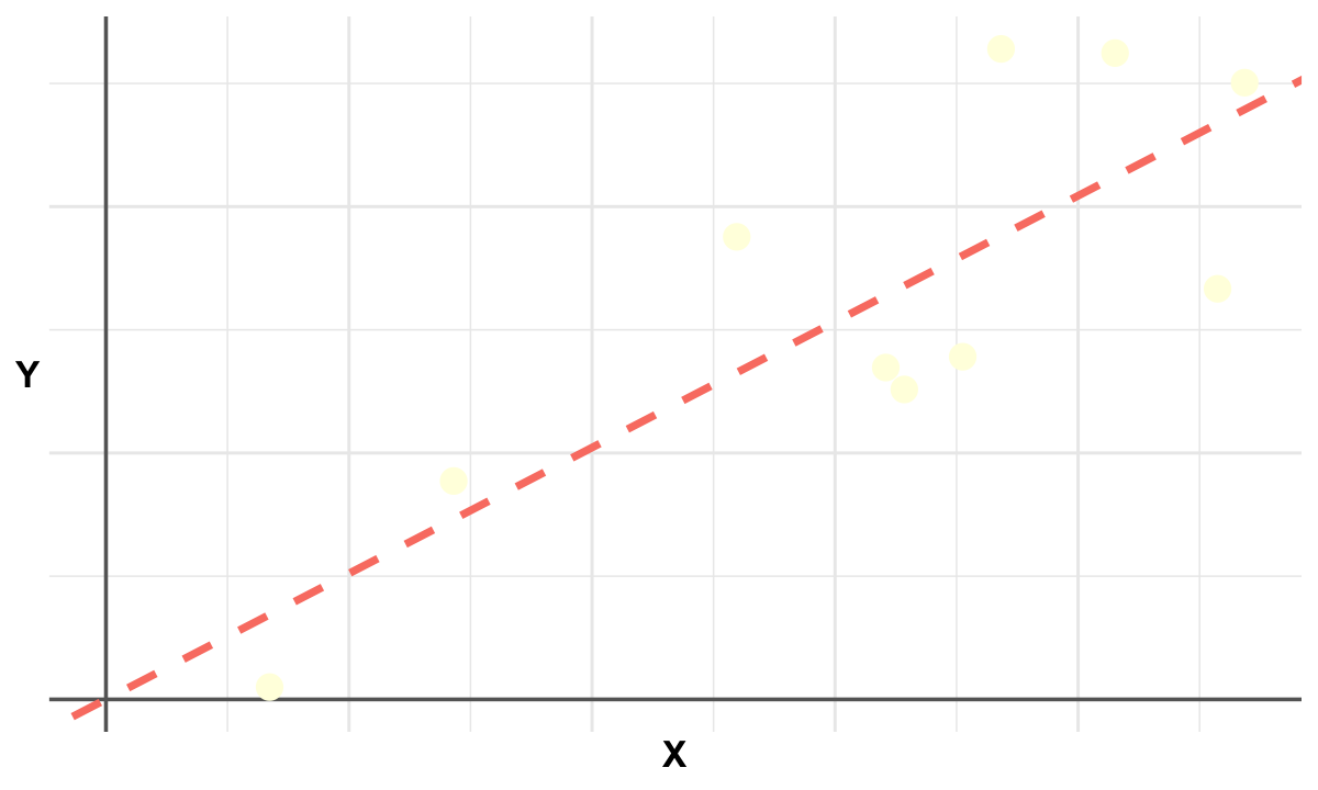
Graphical Summary#
# Load necessary library
library(ggplot2)

options(repr.plot.width = 10, repr.plot.height = 6)

# Generate positive example data
set.seed(42)
x <- runif(10, min = 0, max = 5)  # Positive x values
y <- 0.5 * x + rnorm(10, mean = 0, sd = 1)
y <- y - min(y) + 0.1  # Ensure y is positive
data <- data.frame(x = x, y = y)

# Fit linear model through the origin
model <- lm(y ~ 0 + x, data = data)  # No intercept
beta1 <- coef(model)[1]

# Plot
p <- ggplot(data, aes(x = x, y = y)) +
  geom_hline(yintercept = 0, color = "gray40", linewidth = 1) +
  geom_vline(xintercept = 0, color = "gray40", linewidth = 1) +
  geom_point(color = "lightyellow", size = 6) +  # yellow points
  geom_abline(intercept = 0, slope = beta1, color = "salmon", linetype = "dashed", linewidth = 2) +
  labs(x = "X", y = "Y") +
  theme_minimal(base_size = 18) +
  theme(
    plot.title = element_blank(),  # no title
    axis.title = element_text(size = 20, face = "bold"),
    axis.text = element_blank(),
    axis.ticks = element_blank(),
    axis.title.y = element_text(angle = 0, vjust = 0.5)  # horizontal Y label
  )
print(p)

# Save with transparent background
ggsave("./figures/ordinary_least_squares.png", plot = p,
       width = 6, height = 6,
       bg = "transparent",
       dpi = 300)