Confounder#
A confounder is a variable that influences both the exposure and outcome independently, creating a misleading association between them that doesn’t represent a true causal relationship.
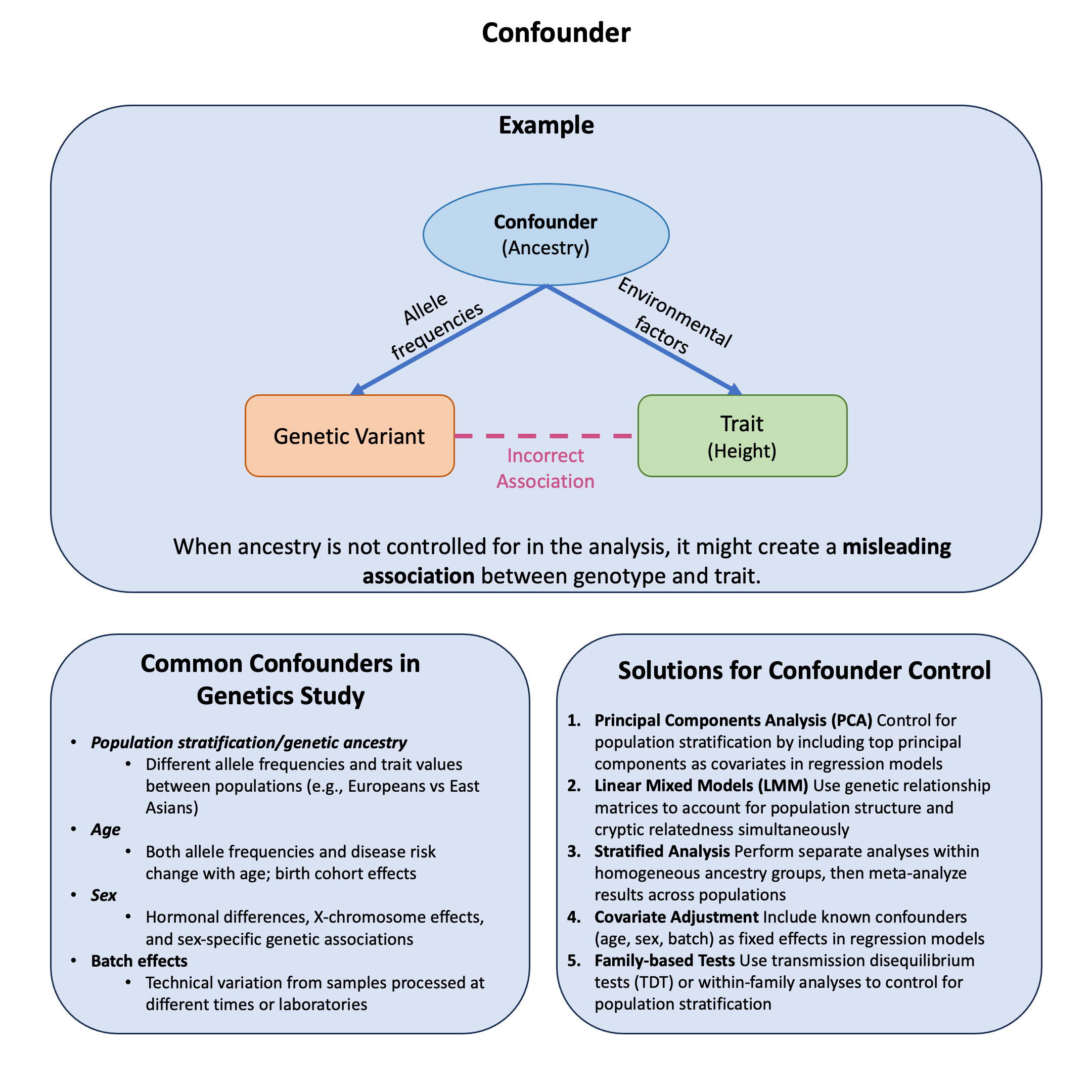
Graphical Summary#
Key Formula#
The key formula for the concept of a confounder is represented in a causal diagram as:
Where:
\(W\) is the confounder variable
\(X\) is the exposure/treatment variable
\(Y\) is the outcome variable
The arrows \((\leftarrow, \rightarrow)\) indicate the direction of causal influence
This diagram illustrates that a confounder (\(W\)) has a direct causal effect on both the exposure (\(X\)) and the outcome (\(Y\)), creating a “backdoor path” between \(X\) and \(Y\) that must be blocked to obtain an unbiased estimate of the causal effect.
Technical Details#
Observed Association vs. True Effect#
When a confounder is present but not controlled:
True Effect: The real biological relationship we want to find
Confounding Bias: The false association created by the confounder
Observed Association: What we actually measure (often misleading!)
The Solution: Control for Confounders#
The most common and practical solution is regression adjustment - simply include confounders as additional variables in your model:
Where \(W_1, W_2, \ldots\) are confounders (e.g., age, ancestry, sex) and \(\beta_1\) is the unbiased effect of genetic variant \(X\).
Here are the common approaches in genetic studies:
Principal Components (Most Common): Control for population structure by including top PCs:
\[ \mathbf{Y} = \mathbf{X}\boldsymbol{\beta} + \text{PC}1 + \text{PC}2 + \text{PC}3 + \text{Age} + \text{Sex} \]Linear Mixed Models: Use genetic relationship matrices for complex population structure:
\[ \mathbf{Y} = \mathbf{X}\boldsymbol{\beta} + \mathbf{g} + \boldsymbol{\epsilon}, \quad \mathbf{g} \sim N(0, \sigma_g^2 \mathbf{G}) \]Stratified Analysis: Analyze each ancestry group separately, then meta-analyze results:
The goal is to block backdoor paths while perserving the direct causal path.
Example#
Recall from our earlier discussion in Example 2 in Lecture: marginal and joint effects about how a genetic variant can appear protective when analyzed alone but harmful when controlling for other factors. This dramatic reversal illustrates confounding - where ancestry affects both variant frequency and disease risk, creating spurious associations.
The key question: How can ancestry confound genetic associations and lead us to completely misinterpret a variant’s true effect?
Setup#
rm(list = ls())
set.seed(9)

N <- 100
# Create a confounding variable (genetic ancestry)
ancestry <- rbinom(N, 1, 0.5)  # 0 = Population A, 1 = Population B

# Generate genotype that's correlated with ancestry
# Population B has higher frequency of risk allele
variant1 <- ifelse(ancestry == 0,
                  rbinom(sum(ancestry == 0), 2, 0.2),  # Pop A: low risk allele frequency
                  rbinom(sum(ancestry == 1), 2, 0.8))  # Pop B: high risk allele frequency

# Check allele frequencies by population
cat("Population A (ancestry=0) mean genotype:", round(mean(variant1[ancestry == 0]), 2), "\n")
cat("Population B (ancestry=1) mean genotype:", round(mean(variant1[ancestry == 1]), 2), "\n")

# Population B has generally lower disease risk (better healthcare/environment)
# But the variant increases risk within each population
baseline_risk <- ifelse(ancestry == 0, 0.8, 0.1)  # Pop A much higher baseline risk
genetic_effect <- 0.1 * variant1  # Variant increases risk in both populations

disease_prob <- baseline_risk + genetic_effect
disease <- rbinom(N, 1, pmin(disease_prob, 1))  # Ensure prob ≤ 1

# Create data frame
data <- data.frame(
  disease = disease,
  variant1 = variant1,
  ancestry = ancestry
)
Population A (ancestry=0) mean genotype: 0.41
Population B (ancestry=1) mean genotype: 1.59
Analysis 1: Ignore Genetic Ancestry#
In Example 2 of Lecture: marginal and joint effects, when the genetic ancestry is not considered in the model, the variant appears to be protective:
# Combining both ancestries and perform analysis
model_combined_ancestries <- glm(disease ~ variant1, data = data, family = binomial)
OR_combined_ancestries <- exp(coef(model_combined_ancestries)[2])
p_combined_ancestries <- summary(model_combined_ancestries)$coefficients[2, 4]

cat("=== ESTIMATED EFFECT (combining genetic ancestries) ===\n")
cat("OR =", round(OR_combined_ancestries, 3), ", p =", round(p_combined_ancestries, 4), "\n")
cat("Interpretation:", ifelse(OR_combined_ancestries > 1, "Detrimental ", "Protective"), "\n")
=== ESTIMATED EFFECT (combining genetic ancestries) ===
OR = 0.394 , p = 4e-04
Interpretation: Protective
Analysis 2: Considering Confounder#
But if we consider the confounder in the model, we will get the correct answer (rather than the Simpson’s paradox that we see in Example 2 in Lecture: marginal and joint effects):
# Combining both ancestries but including ancestry as a covariate
model_controlled <- glm(disease ~ variant1 + ancestry, data = data, family = binomial)
OR_controlled <- exp(coef(model_controlled)[2])
p_controlled <- summary(model_controlled)$coefficients[2, 4]

cat("=== JOINT EFFECT (combining populations, and considering ancestry) ===\n")
cat("OR =", round(OR_controlled, 3), ", p =", round(p_controlled, 4), "\n")
cat("Interpretation:", ifelse(OR_controlled > 1, "Detrimental ", "Protective"), "\n")
=== JOINT EFFECT (combining populations, and considering ancestry) ===
OR = 1.192 , p = 0.6768
Interpretation: Detrimental