Bayesian Normal Mean Model#
The Bayesian normal mean model treats the unknown mean parameter as a normally distributed random variable reflecting our uncertainty, then updates this normal distribution by conditioning on observed data to yield a posterior normal distribution with reduced uncertainty.
Graphical Summary#
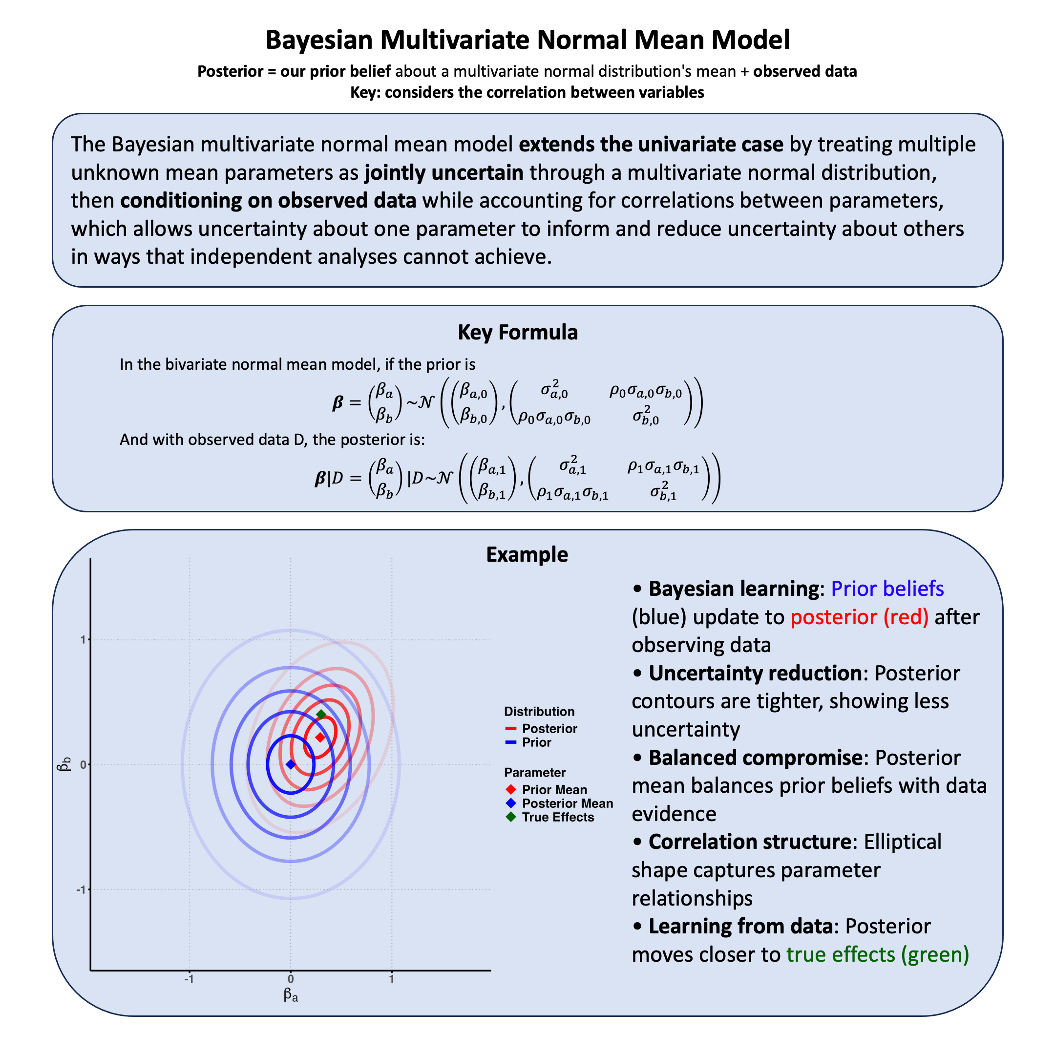
Key Formula#
Under the Bayesian regression setting, we have
with a prior distribution on the regression coefficient: \(\beta \sim \mathcal{N}(\beta_0, \sigma_0^2)\).
\(\mathbf{Y} \in \mathbb{R}^{N}\): phenotype vector of \(N\) samples
\(\mathbf{X} \in \mathbb{R}^{N}\): genotype vector of \(N\) samples (\(\mathbf{X}_i \in \{0, 1, 2\}\) for additive coding)
\(\beta \in \mathbb{R}\): genetic effect size
\(\boldsymbol{\varepsilon} \in \mathbb{R}^{N}\): residual error (i.i.d. Gaussian)
\(\sigma^2\): residual variance
Technical Details#
The Bayesian Perspective#
In Bayesian statistics, parameters are random variables representing our uncertainty, not fixed unknown constants.
Key insight: When we cannot observe something, we treat it as a random variable with a probability distribution quantifying our uncertainty.
Model Setup#
where \(\beta\) is a random variable (we cannot observe the true genetic effect, so we quantify our uncertainty about it).
Prior Distribution#
\(\beta_0\): Best guess before seeing data
\(\sigma_0^2\): How uncertain we are (larger = more uncertain)
The probability density function reflects this uncertainty:
Likelihood#
The likelihood represents what we can condition on - the observed data given our uncertain parameter:
Posterior Distribution#
Using Bayes’ rule, we update our uncertainty given the observed data:
The posterior is:
where:
Note: \(\sigma_1^2 < \sigma_0^2\) always - observing data reduces uncertainty.
Posterior as Weighted Average#
where \(w = \frac{T_1/\sigma^2}{T_1/\sigma^2 + 1/\sigma_0^2}\), \(\hat{\beta}_{\text{data}} = T_2/T_1\), and \(T_1 = \sum_{i=1}^N X_i^2\), \(T_2 = \sum_{i=1}^N X_i Y_i\).
Interpretation:
More data or lower noise (small \(\sigma^2\)) → \(w \approx 1\) (trust data)
Vague prior (large \(\sigma_0^2\)) → \(w \approx 1\) (data dominates)
Strong prior (small \(\sigma_0^2\)) → \(w \approx 0\) (prior dominates)
Example#
When studying genetic effects across many variants, we typically believe most effects are small, some are moderate, and few are large. Rather than assuming each effect is a fixed unknown constant, we model it as a random variable drawn from a distribution.
This leads to a hierarchical structure:
Data level: Phenotype depends on genotype and effect
Effect level: Effect \(\beta\) is random, drawn from a distribution
Hyperparameter level: Distribution parameters estimated from data
Model:
The posterior distribution \(p(\beta | \mathbf{Y})\) shows how plausible each effect size is after combining prior knowledge with observed data.
Why this matters: In genomics with thousands of variants, treating effects as random with shared distributional properties is more realistic than treating each as an independent fixed unknown.
Setup#
First, let’s recreate the exact same genetic data from our previous Lecture: likelihood.
# Clear the environment
rm(list = ls())
library(stats)
library(ggplot2)
set.seed(19)  # For reproducibility

# Generate genotype data for 5 individuals at a single variant
N <- 5
genotypes <- c("CC", "CT", "TT", "CT", "CC")  # Individual genotypes
names(genotypes) <- paste("Individual", 1:N)

# Define alternative allele
alt_allele <- "T"

# Convert to additive genotype coding (count of alternative alleles)
Xraw_additive <- numeric(N)
for (i in 1:N) {
  alleles <- strsplit(genotypes[i], "")[[1]]
  Xraw_additive[i] <- sum(alleles == alt_allele)
}
names(Xraw_additive) <- names(genotypes)

# Standardize genotypes
X <- scale(Xraw_additive, center = TRUE, scale = TRUE)[,1]
# Set true beta and generate phenotype data
true_beta <- 0.4
true_sd <- 1.0

# Generate phenotype with true effect
Y <- X * true_beta + rnorm(N, 0, true_sd)
To apply the Bayesian normal mean model, we need to specify the prior distribution for \(\beta\) and the residual variance \(\sigma^2\). We assume the prior mean is zero (i.e., we have no reason to believe the effect is positive or negative before seeing data):
The prior variance \(\sigma_0^2\) represents how uncertain we are about \(\beta\) before seeing data, and the residual variance \(\sigma^2\) represents how noisy our measurements are. We will estimate both variances from the data using maximum likelihood.
Prior Distribution#
# Define prior distribution
# Prior mean: no prior expectation about direction of effect
beta_0 <- 0

cat("Prior distribution:\n")
cat("beta ~ N(beta_0, sigma_0^2) where beta_0 =", beta_0, "\n")
cat("sigma_0^2 will be estimated from data\n")
Prior distribution:
beta ~ N(beta_0, sigma_0^2) where beta_0 = 0
sigma_0^2 will be estimated from data
Estimating the Variances#
Why estimate variances? We need \(\sigma^2\) and \(\sigma_0^2\) to compute the posterior, but we don’t know their true values. In practice, we estimate them from the data itself.
How? We use the marginal likelihood - the probability of observing our data, averaging over all possible \(\beta\) values:
For our normal-normal model, this has a closed form:
We find the \(\sigma^2\) and \(\sigma_0^2\) that maximize this marginal likelihood.
# Function to compute log marginal likelihood for given parameters
log_marginal_likelihood <- function(params, Y, X) {
  sigma_squared <- params[1]
  sigma_0_squared <- params[2]

  if (sigma_squared <= 0 || sigma_0_squared <= 0) return(-Inf)

  n <- length(Y)

  # Variance matrix: $\sigma^2$I + $\sigma_0^2$XX^T
  var_matrix <- sigma_squared * diag(n) + sigma_0_squared * outer(X, X)

  # Compute log likelihood of multivariate normal
  tryCatch({
    log_det <- determinant(var_matrix, logarithm = TRUE)$modulus
    quad_form <- t(Y) %*% solve(var_matrix) %*% Y

    # Log likelihood (ignoring constants)
    -0.5 * (log_det + quad_form)
  }, error = function(e) -Inf)
}

# Find optimal parameters by maximizing marginal likelihood
optimize_result <- optim(
  par = c(1, 0.5),  # Initial guesses for $\sigma^2$ and $\sigma_0^2$
  fn = function(params) -log_marginal_likelihood(params, Y, X),  # Minimize negative log-likelihood
  method = "L-BFGS-B",
  lower = c(0.01, 0.01),
  upper = c(10, 10)
)

sigma_squared_mle <- optimize_result$par[1]
sigma_0_squared_mle <- optimize_result$par[2]
sigma_mle <- sqrt(sigma_squared_mle)
sigma_0_mle <- sqrt(sigma_0_squared_mle)

print(paste("Estimated sigma^2 (error variance):", round(sigma_squared_mle, 3)))
print(paste("Estimated sigma_0^2 (prior variance):", round(sigma_0_squared_mle, 3)))
[1] "Estimated sigma^2 (error variance): 0.486"
[1] "Estimated sigma_0^2 (prior variance): 0.231"
Posterior Distribution#
With the estimated variances, we can now compute the posterior distribution using the formulas from the Technical Details section above.
# Calculate sufficient statistics
sum_X_squared <- sum(X^2)
sum_XY <- sum(X * Y)

# Posterior parameters using estimated variances and prior mean beta_0
posterior_variance <- 1 / (sum_X_squared/sigma_squared_mle + 1/sigma_0_squared_mle)
posterior_mean <- posterior_variance * (sum_XY/sigma_squared_mle + beta_0/sigma_0_squared_mle)
posterior_sd <- sqrt(posterior_variance)

cat("\nPosterior Results:\n")
cat("beta | D ~ Normal(", round(posterior_mean, 4), ", ", round(posterior_variance, 4), ")\n")
cat("Posterior mean (beta_1):", round(posterior_mean, 4), "\n")
cat("Posterior SD:", round(posterior_sd, 4), "\n")
Posterior Results:
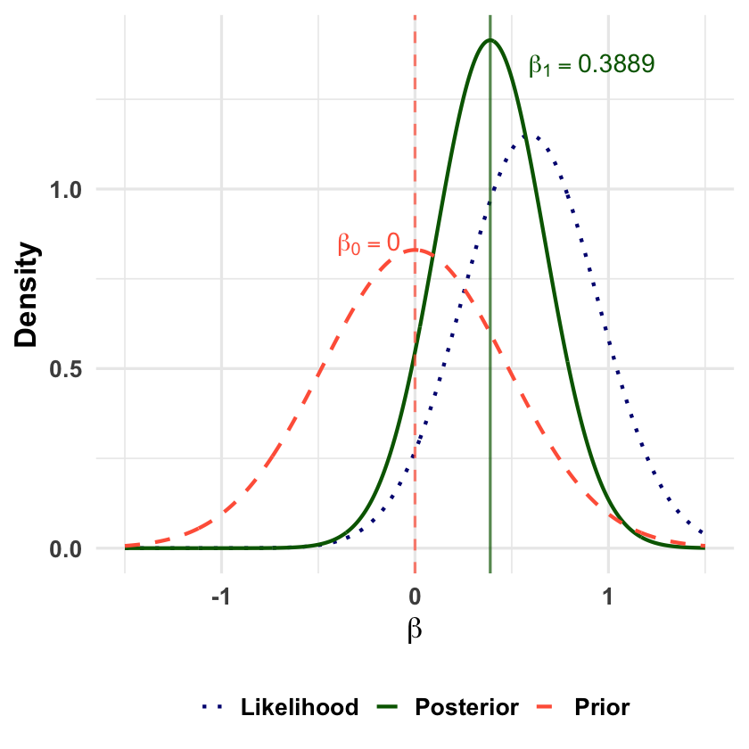
beta | D ~ Normal( 0.3889 , 0.0796 )
Posterior mean (beta_1): 0.3889
Posterior SD: 0.2821
Visualizing the Bayesian Update#
Let’s visualize how observing data updates our beliefs about \(\beta\), shifting from the prior to the posterior distribution.
beta_range <- seq(-1.5, 1.5, length.out = 1000)

# Prior distribution: N(beta_0, sigma_0^2)
prior_density <- dnorm(beta_range, mean = beta_0, sd = sigma_0_mle)

# Likelihood (as a function of beta, treating data as fixed)
# This is proportional to exp(-(sum_X_squared * beta^2 - 2*sum_XY*beta) / (2*sigma^2))
likelihood_unnormalized <- exp(-(sum_X_squared * beta_range^2 - 2*sum_XY*beta_range) / (2*sigma_squared_mle))
# Normalize to make it a proper density
likelihood_density <- likelihood_unnormalized / (sum(likelihood_unnormalized) * (beta_range[2] - beta_range[1]))

# Posterior distribution: N(posterior_mean, posterior_variance)
posterior_density <- dnorm(beta_range, mean = posterior_mean, sd = posterior_sd)

# Combine into data frame
plot_data <- data.frame(
  beta = rep(beta_range, 3),
  density = c(prior_density, likelihood_density, posterior_density),
  distribution = rep(c("Prior", "Likelihood", "Posterior"), each = length(beta_range))
)

# Create the plot
p <- ggplot(plot_data, aes(x = beta, y = density, color = distribution, linetype = distribution)) +
  geom_line(size = 1.2) +
  scale_color_manual(values = c("Prior" = "tomato",
                               "Likelihood" = "#000080",
                               "Posterior" = "darkgreen")) +
  scale_linetype_manual(values = c("Prior" = "dashed",
                                  "Likelihood" = "dotted",
                                  "Posterior" = "solid")) +
  labs(
    y = "Density",
    x = expression(beta),
    color = "Distribution",
    linetype = "Distribution"
  ) +
  theme_minimal(base_size = 20) +
  theme(
    plot.title = element_blank(),
    axis.title.y = element_text(face = "bold"),
    axis.title.x = element_text(face = "bold"),
    axis.text.x = element_text(face = "bold"),
    axis.text.y = element_text(face = "bold"),
    legend.title = element_blank(),
    legend.text = element_text(face = "bold"),
    legend.position = "bottom",
    panel.background = element_rect(fill = "transparent", color = NA),
    plot.background = element_rect(fill = "transparent", color = NA)
  ) +
  guides(color = guide_legend(override.aes = list(size = 1.5)))

# Add vertical lines for means and annotations
p <- p +
  geom_vline(xintercept = beta_0, color = "tomato", linetype = "dashed", alpha = 0.7) +
  geom_vline(xintercept = posterior_mean, color = "darkgreen", linetype = "solid", alpha = 0.7) +
  annotate("text", x = beta_0-0.5, y = max(plot_data$density) * 0.6,
           label = paste0("beta[0]==", beta_0), color = "tomato", size = 6, fontface = "bold", hjust = -0.3, parse = TRUE) +
  annotate("text", x = posterior_mean, y = max(plot_data$density) * 0.95,
           label = paste0("beta[1]==", round(posterior_mean, 4)), color = "darkgreen", size = 6, fontface = "bold", hjust = -0.3, parse = TRUE)

# Display plot
print(p)
ggsave("./figures/Bayesian_normal_mean_model.png", plot = p,
      width = 10, height = 6, dpi = 300, bg = "transparent")