Genetic Relationship Matrix#
Genetic relationship matrix (GRM) captures how related individuals are to each other at the genomic level by calculating the correlation in standardized genotypes across the genome to quantify the genetic similarity between every pair of individuals in the population.
Graphical Summary#
Key Formula#
Genomic Relationship Matrix (GRM) is a standardized version of the kinship matrix that accounts for allele frequencies. One common formulation is:
Where:
\(\mathbf{X}\) is the scaled genotype matrix of \(N\) individuals and \(M\) genetic variants.
\(\mathbf{G}\) is an \( N \times N \) matrix capturing the pairwise genetic relationships.
Technical Details#
Relationship to Kinship#
Kinship quantifies the expected proportion of genome shared identical-by-descent (IBD) from recent common ancestors. Traditional kinship assumes known pedigrees, but IBD can also be estimated directly from genetic data. Parent-offspring pairs share 50% IBD; unrelated individuals share negligible IBD despite ~99.9% overall sequence similarity among humans.
The GRM instead measures realized genetic similarity directly from observed genotypes, without requiring pedigree information. Rather than tracking inheritance from known ancestors, it asks: “Based on thousands of genetic variants, how similar are these two individuals’ genomes?”
Why rare variants should matter more?#
The GRM weights variants by their informativeness. If everyone in the population carries allele A at a locus, observing that two individuals both have A reveals nothing about their relationship. But if only 2% carry the rare allele B, two individuals sharing B is highly informative. By standardizing variants using population allele frequencies, the GRM appropriately weights rare shared alleles more heavily than common ones.
Scaling Properties#
Because variants are standardized to unit variance across individuals (not within individuals), diagonal elements of G aren’t necessarily 1. Each diagonal value indicates how genetically “typical” that individual is relative to the population mean.
Why GRM for statistical genetics?#
Unlike kinship coefficients that capture only recent familial relationships, the GRM captures all sources of genetic similarity - both close relatedness and subtle population structure among seemingly unrelated individuals. This makes it essential for:
Mixed models accounting for population stratification and cryptic relatedness
Heritability estimation in unrelated cohorts
Genomic prediction without pedigree information
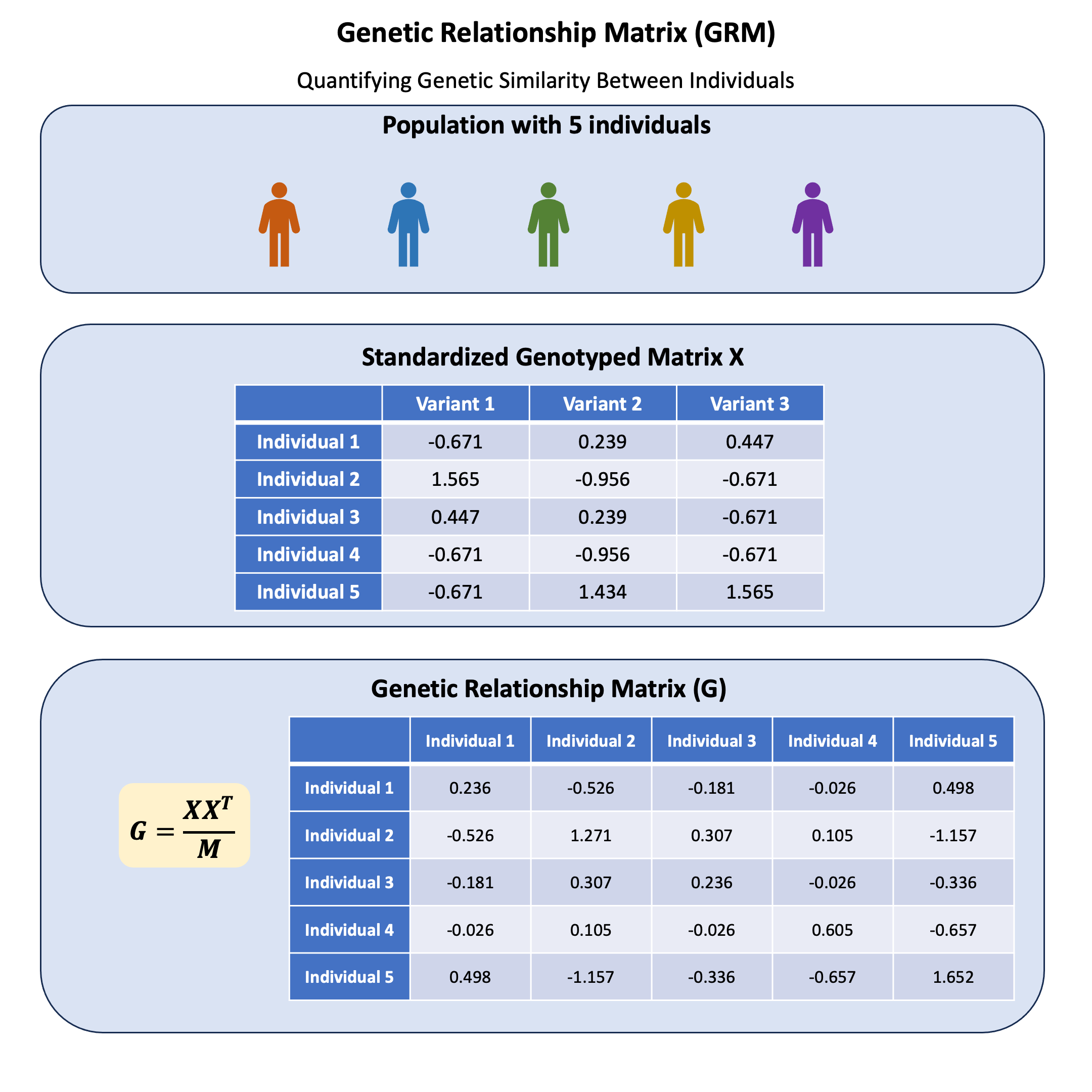
Example#
Now let’s compute the GRM from our toy dataset of 5 individuals and 3 variants. Which individuals appear most genetically similar? Do any look related? What do the GRM values actually tell us?
Let’s calculate the GRM step by step and interpret each element.
Setup#
# Clear the environment
rm(list = ls())

# Define genotypes for 5 individuals at 3 variants
# These represent actual alleles at each position
# For example, Individual 1 has genotypes: CC, CT, AT
genotypes <- c(
 "CC", "CT", "AT",  # Individual 1
 "TT", "TT", "AA",  # Individual 2
 "CT", "CT", "AA",  # Individual 3
 "CC", "TT", "AA",  # Individual 4
 "CC", "CC", "TT"   # Individual 5
)
# Reshape into a matrix
N = 5
M = 3
geno_matrix <- matrix(genotypes, nrow = N, ncol = M, byrow = TRUE)
rownames(geno_matrix) <- paste("Individual", 1:N)
colnames(geno_matrix) <- paste("Variant", 1:M)

alt_alleles <- c("T", "C", "T")

# Convert to raw genotype matrix using the additive model
Xraw_additive <- matrix(0, nrow = N, ncol = M) # count number of non-reference alleles

rownames(Xraw_additive) <- rownames(geno_matrix)
colnames(Xraw_additive) <- colnames(geno_matrix)

for (i in 1:N) {
  for (j in 1:M) {
    alleles <- strsplit(geno_matrix[i,j], "")[[1]]
    Xraw_additive[i,j] <- sum(alleles == alt_alleles[j])
  }
}

X <- scale(Xraw_additive, center = TRUE, scale = TRUE)
Scaling \(\mathbf{X}\)#
The scaled genotype matrix X (scaled with respective for column) is:
X
| Variant 1 | Variant 2 | Variant 3 | |
|---|---|---|---|
| Individual 1 | -0.6708204 | 0.2390457 | 0.4472136 |
| Individual 2 | 1.5652476 | -0.9561829 | -0.6708204 |
| Individual 3 | 0.4472136 | 0.2390457 | -0.6708204 |
| Individual 4 | -0.6708204 | -0.9561829 | -0.6708204 |
| Individual 5 | -0.6708204 | 1.4342743 | 1.5652476 |
Calculating GRM#
The GRM can be calculated as:
# calculate the GRM
GRM = (X %*% t(X)) / M
GRM
| Individual 1 | Individual 2 | Individual 3 | Individual 4 | Individual 5 | |
|---|---|---|---|---|---|
| Individual 1 | 0.23571429 | -0.5261905 | -0.18095238 | -0.02619048 | 0.4976190 |
| Individual 2 | -0.52619048 | 1.2714286 | 0.30714286 | 0.10476190 | -1.1571429 |
| Individual 3 | -0.18095238 | 0.3071429 | 0.23571429 | -0.02619048 | -0.3357143 |
| Individual 4 | -0.02619048 | 0.1047619 | -0.02619048 | 0.60476190 | -0.6571429 |
| Individual 5 | 0.49761905 | -1.1571429 | -0.33571429 | -0.65714286 | 1.6523810 |