Expectation-Maximum Algorithm#
The EM algorithm breaks an impossible optimization problem into two manageable steps that feed into each other: first calculating what the hidden data probably looks like given current parameter estimates, then finding better parameters by treating those probabilistic guesses as if they were observations.
Graphical Summary#
Key Formula#
Given a statistical model parameterized by \(\theta\) that generates observed data \(\mathbf{X}\) and unobserved latent data \(\mathbf{Z}\), the goal is to find the maximum likelihood estimate (MLE) \(\hat{\theta}_\text{MLE}\) by maximizing the marginal likelihood:
This integral is often intractable because \(\mathbf{Z}\) is unobserved and its distribution depends on the unknown \(\theta\).
The EM algorithm finds \(\hat{\theta}_\text{MLE}\) iteratively through two steps:
E-step (Expectation): Compute the expected log-likelihood of \(\theta\) with respect to the conditional distribution of \(\mathbf{Z}\) given \(\mathbf{X}\) and current parameter estimate \(\theta^{(t)}\):
M-step (Maximization): Find parameters that maximize \(Q\):
Technical Details#
Why EM Works: The Monotonic Increase Guarantee#
Why does maximizing \(Q(\theta \mid \theta^{(t)})\) increase the observed-data log-likelihood \(\ell(\theta; \mathbf{X}) = \log P(\mathbf{X} \mid \theta)\)?
The observed-data log-likelihood can be decomposed as:
where \(H(\theta \mid \theta^{(t)})\) is the conditional entropy of the latent variables:
The entropy term is maximized when \(\theta = \theta^{(t)}\). Therefore, each EM iteration increases (or maintains) the observed-data log-likelihood (complete proof can be found here).
Practical Implementation#
E-Step: Computing Responsibilities
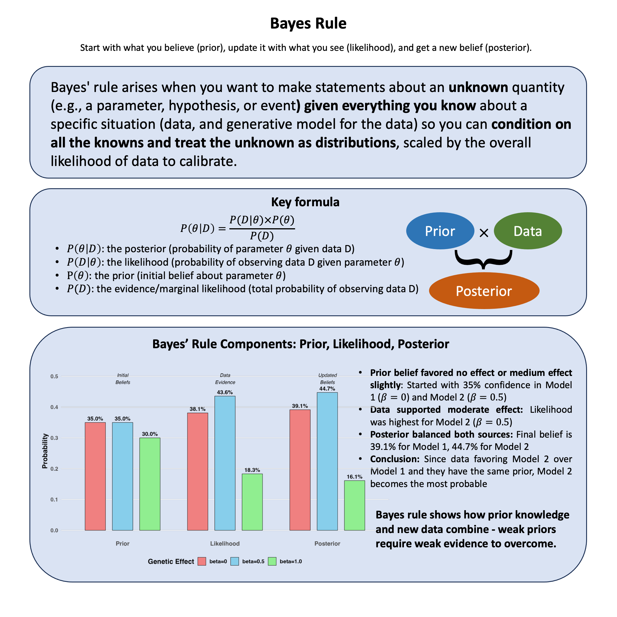
For each observation \(i\) and latent state \(k\), compute the posterior probability using Bayes’ rule (introduced in Lecture: Bayes’ rule):
These responsibilities \(w_{ik}^{(t)}\) represent the posterior probability that observation \(i\) belongs to latent state \(k\).
M-Step: Maximizing the Q-Function
Find parameters that best explain the data, using responsibilities as weights:
This is weighted maximum likelihood estimation, often with closed-form solutions like weighted averages.
Further Reading#
For more detailed examples and alternative perspectives on the EM algorithm, we recommend the following references from Matthew Stephens:
Example#
Suppose we’re studying a genetic variant and want to estimate its minor allele frequency (MAF). We’ve genotyped \(N\) individuals, but our sequencing technology makes errors. Some individuals who are truly homozygous AA might be called as AB or BB, and vice versa.
The problem: If we naively count alleles from observed genotypes, our MAF estimate will be biased. How can we estimate both the true MAF and error rate simultaneously?
We apply the EM algorithm to solve this problem. The true genotypes are our missing data – if we knew them, estimating MAF and error rate would be trivial. EM handles this uncertainty.
Set Up#
rm(list=ls())
library(ggplot2)
library(dplyr)
set.seed(581)
# True parameters
f_true <- 0.3 # true MAF
epsilon_true <- 0.05 # true error rate
n <- 10000 # sample size

# Step 1: Generate true genotypes according to Hardy-Weinberg equilibrium
# P(g=0) = (1-f)^2, P(g=1) = 2f(1-f), P(g=2) = f^2
hw_probs <- c((1-f_true)^2, 2*f_true*(1-f_true), f_true^2)
true_genotypes <- sample(0:2, size = n, replace = TRUE, prob = hw_probs)

# Step 2: Add genotyping errors
observed_genotypes <- true_genotypes  # Start with true genotypes
errors <- runif(n) < epsilon_true     # Which observations have errors?

# For observations with errors, randomly assign a genotype
for (i in which(errors)) {
  observed_genotypes[i] <- sample(0:2, size = 1)
}

# Create a data frame
data <- data.frame(
  individual = 1:n,
  true_genotype = true_genotypes,
  observed_genotype = observed_genotypes,
  error = errors
)

# Summary
cat("True MAF:", f_true, "\n")
cat("Naive MAF estimate:", sum(observed_genotypes) / (2*n), "\n")
cat("Number of errors introduced:", sum(errors), "\n")
Attaching package: ‘dplyr’


The following objects are masked from ‘package:stats’:

    filter, lag


The following objects are masked from ‘package:base’:

    intersect, setdiff, setequal, union
True MAF: 0.3
Naive MAF estimate: 0.31315
Number of errors introduced: 494
EM Algorithm#
Theory#
Observed data: \(\mathbf{D} = (D_1, \ldots, D_N)\) where \(D_i \in \{0, 1, 2\}\)
Missing data: \(\mathbf{G} = (G_1, \ldots, G_N)\) where \(G_i \in \{0, 1, 2\}\) (true genotypes)
Parameters: \(\theta = (f, \epsilon)\) where \(f\) is the true MAF and \(\epsilon\) is the genotyping error rate
The Hardy-Weinberg equilibrium (introduced in Lecture: Hardy Weinberg equilibrium) tells us that the allele frequency remains constant across generations in a population.
When there is genotyping error, we assume that with probability \(\epsilon\), a genotyping error occurs and the observed genotype is randomly assigned to {0, 1, 2} with equal probability \(\frac{1}{3}\) each. When the true genotype is \(j\), observing the correct genotype \(j\) can happen two ways: no error (probability \(1-\epsilon\)) or an error that randomly lands on \(j\) (with probability \(\frac{1}{3}\epsilon\)), giving total probability \(1 - \frac{2\epsilon}{3}\). Observing an incorrect genotype \(k \neq j\) only happens through errors, with probability \(\frac{\epsilon}{3}\).
Implementation#
# Function to compute error model probabilities
p_obs_given_true <- function(d, g, epsilon) {
  # P(observed = d | true = g, epsilon)
  if (d == g) {
    return(1 - 2*epsilon/3)
  } else {
    return(epsilon/3)
  }
}

# Function to compute Hardy-Weinberg probabilities
p_true_given_f <- function(g, f) {
  # P(true genotype = g | MAF = f)
  if (g == 0) return((1-f)^2)
  if (g == 1) return(2*f*(1-f))
  if (g == 2) return(f^2)
}

# E-Step: Compute responsibilities
e_step <- function(observed, f, epsilon) {
  n <- length(observed)
  w <- matrix(0, nrow = n, ncol = 3)  # responsibilities for genotypes 0, 1, 2

  for (i in 1:n) {
    d_i <- observed[i]

    # Compute unnormalized weights for each possible true genotype
    for (g in 0:2) {
      w[i, g+1] <- p_obs_given_true(d_i, g, epsilon) * p_true_given_f(g, f)
    }

    # Normalize
    w[i, ] <- w[i, ] / sum(w[i, ])
  }

  return(w)
}

# M-Step: Update parameters
m_step <- function(observed, w) {
  n <- nrow(w)

  # Update f (MAF)
  # Expected number of B alleles = sum over individuals of (1*w_i1 + 2*w_i2)
  f_new <- sum(w[, 2] + 2*w[, 3]) / (2*n)

  # Update epsilon (error rate)
  # Expected number of correct calls = sum over individuals of w_{i,d_i}
  correct_calls <- sapply(1:n, function(i) w[i, observed[i] + 1])
  epsilon_new <- (3/2) * (n - sum(correct_calls)) / n

  return(list(f = f_new, epsilon = epsilon_new))
}

# Complete EM algorithm
em_algorithm <- function(observed, f_init, epsilon_init, max_iter = 1000, tol = 1e-6) {
  f <- f_init
  epsilon <- epsilon_init

  # Store history
  history <- data.frame(
    iteration = 0,
    f = f,
    epsilon = epsilon,
    log_likelihood = NA
  )

  for (iter in 1:max_iter) {
    # E-step
    w <- e_step(observed, f, epsilon)

    # M-step
    params <- m_step(observed, w)
    f_new <- params$f
    epsilon_new <- params$epsilon

    # Store history
    history <- rbind(history, data.frame(
      iteration = iter,
      f = f_new,
      epsilon = epsilon_new,
      log_likelihood = NA
    ))

    # Check convergence
    if (abs(f_new - f) < tol && abs(epsilon_new - epsilon) < tol) {
      cat("Converged after", iter, "iterations\n")
      break
    }

    f <- f_new
    epsilon <- epsilon_new
  }

  return(list(
    f = f,
    epsilon = epsilon,
    history = history,
    responsibilities = w
  ))
}
Performing EM Algorithm#
# Initialize parameters
# Use naive estimates as starting values
f_init <- sum(observed_genotypes) / (2*n)
epsilon_init <- 0.01

cat("Initial values:\n")
cat("f_init =", f_init, "\n")
cat("epsilon_init =", epsilon_init, "\n\n")

# Run EM
results <- em_algorithm(observed_genotypes, f_init, epsilon_init)
Initial values:
f_init = 0.31315
epsilon_init = 0.01
Converged after 362 iterations
Results and Visualization#
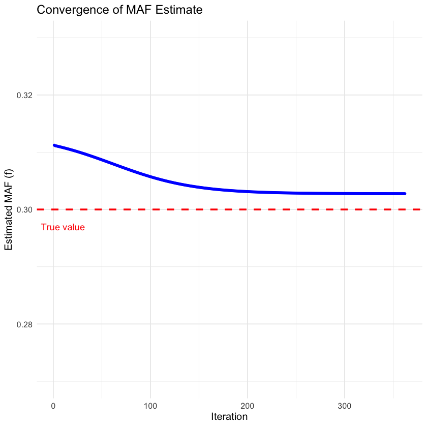
Now let’s visualize how the EM algorithm converged to the final estimates and examine the quality of the results.
The convergence plots below show how the MAF and error rate estimates evolved across iterations. Note that the MAF estimate converges quickly and gets close to the true value, and the error rate estimate also converges.
cat("\nFinal estimates:\n")
cat("Estimated MAF (f) =", results$f, "(true value:", f_true, ")\n")
cat("Estimated error rate (epsilon) =", results$epsilon, "(true value:", epsilon_true, ")\n")
Final estimates:
Estimated MAF (f) = 0.3027583 (true value: 0.3 )
Estimated error rate (epsilon) = 0.05268373 (true value: 0.05 )
p1 <- ggplot(results$history[-1, ], aes(x = iteration, y = f)) +
  geom_point(color = "blue", size = 1) +
  geom_hline(yintercept = f_true, linetype = "dashed", color = "red", linewidth = 1) +
  ylim(f_true*0.9, f_true*1.1) +
  annotate("text", x = 10, y = f_true * 0.99,
           label = "True value", color = "red") +
  labs(title = "Convergence of MAF Estimate",
       x = "Iteration",
       y = "Estimated MAF (f)") +
  theme_minimal() +
  theme(text = element_text(size = 12))
p1
comparison <- data.frame(
  Parameter = c("MAF (f)", "Error rate (ε)"),
  True_Value = c(f_true, epsilon_true),
  EM_Estimate = c(results$f, results$epsilon),
  Absolute_Error = c(abs(results$f - f_true), abs(results$epsilon - epsilon_true))
)
comparison
| Parameter | True_Value | EM_Estimate | Absolute_Error |
|---|---|---|---|
| <chr> | <dbl> | <dbl> | <dbl> |
| MAF (f) | 0.30 | 0.30275828 | 0.002758281 |
| Error rate (ε) | 0.05 | 0.05268373 | 0.002683732 |