Getting started

mfsusieR is the multi-outcome, functional regression generalization of susieR::susie(). It provides two main functions:

fsusie(Y, X, pos = NULL, ...) for fine-mapping a single response. Y may be scalar (T = 1, recovers susieR::susie()) or functional (T > 1, the single-outcome functional SuSiE model).
mfsusie(X, Y, pos = NULL, ...) for fine-mapping multiple responses jointly. Y is a list of length M outcomes; each element is a matrix n x T_m (with T_m = 1 for scalar outcomes).

Both functions return an object of class c("mfsusie", "susie") with the standard SuSiE fields (alpha, mu, mu2, lbf, KL, sigma2, elbo, pip, sets, niter, converged).

library(mfsusieR)
library(susieR)
set.seed(1)

Both fits return raw inverse-DWT effect curves through coef(). For a smoothed position-space curve with a pointwise credible band (and, for the HMM smoother, a per-position lfsr curve), post-process with mf_post_smooth(). Four methods are available: (i) "TI" (the default), translation-invariant wavelet denoising via cycle spinning; (ii) "scalewise", per-scale soft-thresholding of the wavelet posterior; (iii) "HMM", a hidden Markov model on per-position regression residuals with a per-position lfsr curve; (iv) "smash", delegates to smashr::smash.gaus. See vignette("post_processing") for the walk-through and the comparison workflow when several smoothers coexist on one fit.

A small `fsusie()` example (single outcome, functional)

Simulate one functional response on a length-32 grid with two causal variables.

n <- 200; p <- 50; T_m <- 32
X <- matrix(rnorm(n * p), nrow = n)
beta <- numeric(p); beta[c(5, 17)] <- c(1.2, -0.8)
Y <- X %*% matrix(rep(beta, T_m), nrow = p) +
     matrix(rnorm(n * T_m, sd = 0.4), nrow = n)

fit_f <- fsusie(Y, X)
#> iter          ELBO       delta   sigma2      mem      V  extras
#>    1    -8987.2658           -   [0.995, 0.997, 1.000]   0.15 GB  [2.67e-02, 1.16e-02, 0 x 3]  pi_null=[0.94, 1.00]
#> iter   2: max|d(alpha,PIP)|=2.83e-10, V=[2.67e-02, 1.20e-02, 0 x 3] -- converged (alpha_pip_fixed_point) [mem: 0.16 GB]
#> [L_greedy] 1 round, greedy_lbf_cutoff=0.100, final L=5
#> round  L     min(lbf)   action
#> 1      5     0.000      saturated
fit_f$pip[c(5, 17)]
#> [1] 1 1
length(fit_f$sets$cs)
#> [1] 2

fsusie() is a thin wrapper around mfsusie(X, list(Y), list(pos), ...); the two fits are bit-identical. mfsusie_plot() works on either:

plot_dims_f <- mfsusie_plot_dimensions(fit_f)

mfsusie_plot(fit_f)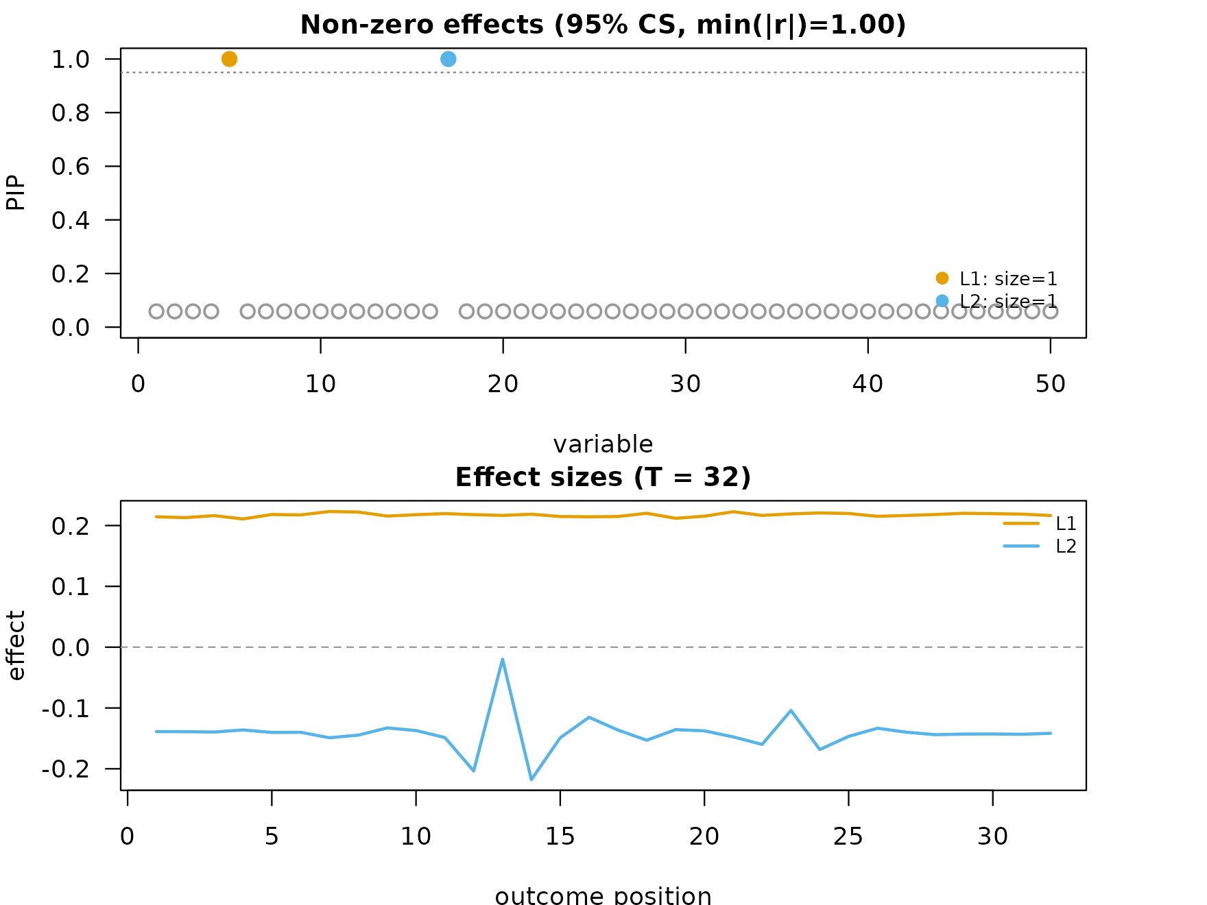

A small `mfsusie()` example (multi-outcome)

Same X and effect vector, two functional outcomes at different resolutions plus one scalar outcome.

T_per <- c(32L, 64L)
Y_func <- lapply(T_per, function(T_m) {
  X %*% matrix(rep(beta, T_m), nrow = p) +
    matrix(rnorm(n * T_m, sd = 0.4), nrow = n)
})
Y_scalar <- as.numeric(X %*% beta + rnorm(n, sd = 0.4))
Y_list <- c(Y_func, list(matrix(Y_scalar, ncol = 1)))

fit_m <- mfsusie(X, Y_list)
#> iter          ELBO       delta   sigma2      mem      V  extras
#>    1   -27230.2239           -   [0.995, 0.997, 1.000]   0.16 GB  [2.46e-01, 1.20e-01, 3.67e-04, 0 x 2]  pi_null=[0.13, 1.00]
#> iter   2: max|d(alpha,PIP)|=8.02e-02, V=[2.46e-01, 1.20e-01, 5.56e-04, 0 x 2] [mem: 0.16 GB]
#> iter   3: max|d(alpha,PIP)|=8.42e-02, V=[2.46e-01, 1.20e-01, 5.71e-04, 0 x 2] [mem: 0.16 GB]
#> iter   4: max|d(alpha,PIP)|=8.44e-02, V=[2.46e-01, 1.20e-01, 5.71e-04, 0 x 2] [mem: 0.16 GB]
#> iter   5: max|d(alpha,PIP)|=2.33e-05, V=[2.46e-01, 1.20e-01, 5.71e-04, 0 x 2] -- converged (alpha_pip_fixed_point) [mem: 0.16 GB]
#> [L_greedy] 1 round, greedy_lbf_cutoff=0.100, final L=5
#> round  L     min(lbf)   action
#> 1      5     0.000      saturated
fit_m$pip[c(5, 17)]
#> [1] 1 1
length(fit_m$sets$cs)
#> [1] 2

mu[[l]][[m]] is a p x T_basis[m] matrix of per-effect posterior means on each outcome; predict() and coef() invert the wavelet transform to position space transparently. mfsusie_plot() tiles one effect-curve panel per outcome with the PIPs in the top-left slot:

plot_dims_m <- mfsusie_plot_dimensions(fit_m)

mfsusie_plot(fit_m)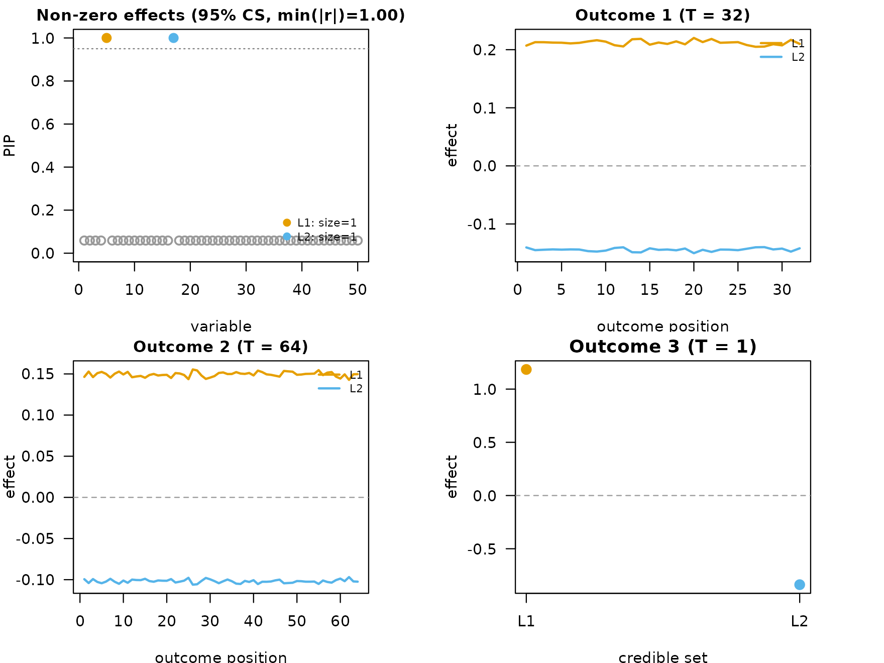

coef(fit_m) returns a per-outcome list of L x T_basis[m] matrices on the original X scale: row l of element m is the inverse-DWT’d effect curve for effect l on outcome m.

cf <- coef(fit_m)
length(cf)                             # one per outcome (M)
#> [1] 3
dim(cf[[1L]])                          # L x T_basis[1]
#> [1]  5 32

predict(fit_m, newx = X_new) returns the fitted per-position response on a fresh genotype matrix:

X_new <- matrix(rnorm(20 * p), 20, p)
pr    <- predict(fit_m, newx = X_new)
length(pr); dim(pr[[1L]])              # n_new x T_basis[m]
#> [1] 3
#> [1] 20 32

# Plot the predicted curve for the first outcome on the first
# four held-out samples.
matplot(t(pr[[1L]][seq_len(4L), ]), type = "l", lty = 1,
        xlab = "position", ylab = "predicted Y",
        main = "predict.mfsusie() on outcome 1")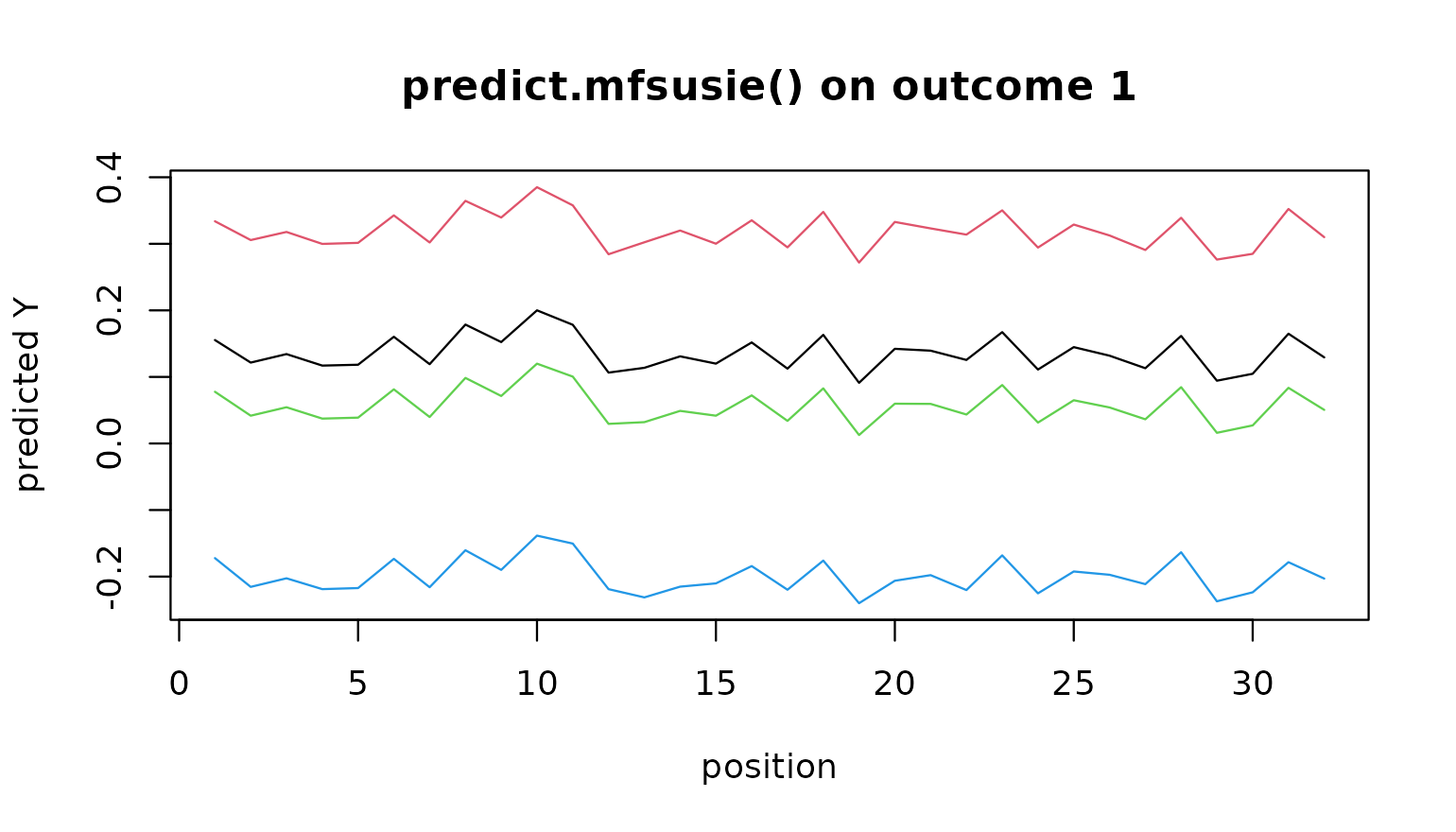

Inspecting a fit

summary() prints a one-screen overview of any mfsusie / fsusie fit: dimensions, IBSS iterations and convergence, the final ELBO, the credible-set table (per-CS size, purity, lead SNP), top PIPs, and the mixture-prior null-mass summary across all (outcome, scale) cells.

summary(fit_f)
#> mfsusie summary: p=50, L=5, M=1, converged in 2 iter
#>   T_basis per outcome: (32)
#>   Final ELBO: -8985.1093
#>   Mixture null-mass across (m, s): min=0.941, median=1.000, max=1.000
#>   Credible sets:
#>     CS 1: size=1, purity=1.000, variables=5
#>     CS 2: size=1, purity=1.000, variables=17

The same call works on the multi-outcome fit and shows the same structure with the per-outcome T_basis:

summary(fit_m)
#> mfsusie summary: p=50, L=5, M=3, converged in 5 iter
#>   T_basis per outcome: (32, 64, 1)
#>   Final ELBO: -27049.6902
#>   Mixture null-mass across (m, s): min=0.130, median=1.000, max=1.000
#>   Credible sets:
#>     CS 1: size=1, purity=1.000, variables=5
#>     CS 2: size=1, purity=1.000, variables=17

Numerical equivalence with `susieR::susie`

For scalar Y (T = 1), with a length-1 prior_variance_grid, null_prior_init = 0, and estimate_prior_variance = FALSE, the per-(outcome, scale) mixture collapses to a single fixed Gaussian effect prior and the per-(scale, outcome) variance structure collapses to one scalar per outcome. In that parameter regime mfsusie() reduces to susieR::susie() bit-for-bit. We use this degenerate equivalence as a sanity check that the multi-outcome wavelet plumbing introduces no per-iteration drift on top of the susieR backbone.

y_scalar <- as.numeric(X %*% beta + rnorm(n, sd = 0.4))
y <- (y_scalar - mean(y_scalar)) / sd(y_scalar)

fit_s <- susie(X, y, L = 5,
               scaled_prior_variance      = 0.2,
               estimate_prior_variance    = FALSE,
               estimate_residual_variance = TRUE,
               max_iter = 100, tol = 1e-8)

fit_d <- mfsusie(X, list(matrix(y, ncol = 1)),
                 L                        = 5,
                 prior_variance_grid      = 0.2,
                 prior_variance_scope     = "per_outcome",
                 null_prior_init        = 0,
                 residual_variance_scope  = "per_outcome",
                 estimate_prior_variance = FALSE,
                 L_greedy                 = NULL,
                 max_iter = 100, tol = 1e-8,
                 verbose = FALSE)

# Element-wise agreement on every numeric field.
max(abs(fit_d$alpha - fit_s$alpha))
#> [1] 8.755743e-05
max(abs(fit_d$pip   - fit_s$pip))
#> [1] 6.64687e-06
max(abs(fit_d$sigma2[[1]] - fit_s$sigma2))
#> [1] 1.239571e-08
max(abs(fit_d$lbf   - fit_s$lbf))
#> [1] 0.0001700982
max(abs(fit_d$KL    - fit_s$KL))
#> [1] 0.0001555593
abs(tail(fit_d$elbo, 1) - tail(fit_s$elbo, 1))
#> [1] 9.323358e-09
identical(fit_d$niter, fit_s$niter)
#> [1] FALSE

The credible-set memberships are also identical:

identical(lapply(fit_d$sets$cs, sort),
          lapply(fit_s$sets$cs, sort))
#> [1] TRUE

All seven comparisons agree at machine precision and the credible sets coincide.

Where to next

Single-outcome applications: Single-outcome intro, covariate adjustment, colocalization, DNAm case study, why functional.
Multi-outcome applications: Multi-outcome intro, long-running fits.
Smoothing the recovered effect curves: post-processing.

Session info

This is the version of R and the packages that were used to generate these results.

sessionInfo()
#> R version 4.4.3 (2025-02-28)
#> Platform: x86_64-conda-linux-gnu
#> Running under: Ubuntu 24.04.4 LTS
#> 
#> Matrix products: default
#> BLAS/LAPACK: /home/runner/work/mfsusieR/mfsusieR/.pixi/envs/r44/lib/libopenblasp-r0.3.32.so;  LAPACK version 3.12.0
#> 
#> locale:
#>  [1] LC_CTYPE=C.UTF-8       LC_NUMERIC=C           LC_TIME=C.UTF-8       
#>  [4] LC_COLLATE=C.UTF-8     LC_MONETARY=C.UTF-8    LC_MESSAGES=C.UTF-8   
#>  [7] LC_PAPER=C.UTF-8       LC_NAME=C              LC_ADDRESS=C          
#> [10] LC_TELEPHONE=C         LC_MEASUREMENT=C.UTF-8 LC_IDENTIFICATION=C   
#> 
#> time zone: Etc/UTC
#> tzcode source: system (glibc)
#> 
#> attached base packages:
#> [1] stats     graphics  grDevices utils     datasets  methods   base     
#> 
#> other attached packages:
#> [1] susieR_0.16.1  mfsusieR_0.0.2
#> 
#> loaded via a namespace (and not attached):
#>  [1] sass_0.4.10           generics_0.1.4        ashr_2.2-63          
#>  [4] lattice_0.22-9        digest_0.6.39         magrittr_2.0.5       
#>  [7] evaluate_1.0.5        grid_4.4.3            RColorBrewer_1.1-3   
#> [10] fastmap_1.2.0         plyr_1.8.9            jsonlite_2.0.0       
#> [13] Matrix_1.7-5          reshape_0.8.10        mixsqp_0.3-54        
#> [16] scales_1.4.0          truncnorm_1.0-9       invgamma_1.2         
#> [19] textshaping_1.0.5     jquerylib_0.1.4       cli_3.6.6            
#> [22] crayon_1.5.3          zigg_0.0.2            rlang_1.2.0          
#> [25] deconvolveR_1.2-1     LaplacesDemon_16.1.8  splines_4.4.3        
#> [28] cachem_1.1.0          yaml_2.3.12           otel_0.2.0           
#> [31] ebnm_1.0-55           tools_4.4.3           SQUAREM_2026.1       
#> [34] parallel_4.4.3        dplyr_1.2.1           wavethresh_4.7.3     
#> [37] ggplot2_4.0.3         Rfast_2.1.5.2         vctrs_0.7.3          
#> [40] R6_2.6.1              matrixStats_1.5.0     lifecycle_1.0.5      
#> [43] fs_2.1.0              htmlwidgets_1.6.4     MASS_7.3-65          
#> [46] trust_0.1-9           ragg_1.5.2            irlba_2.3.7          
#> [49] pkgconfig_2.0.3       desc_1.4.3            RcppParallel_5.1.11-2
#> [52] pkgdown_2.2.0         bslib_0.10.0          pillar_1.11.1        
#> [55] gtable_0.3.6          glue_1.8.1            Rcpp_1.1.1-1.1       
#> [58] systemfonts_1.3.2     xfun_0.57             tibble_3.3.1         
#> [61] tidyselect_1.2.1      dichromat_2.0-0.1     knitr_1.51           
#> [64] farver_2.1.2          htmltools_0.5.9       rmarkdown_2.31       
#> [67] compiler_4.4.3        S7_0.2.2              horseshoe_0.2.0

Gao Wang, Anjing Liu and William Denault

A small fsusie() example (single outcome, functional)