Joint multi-outcome fine-mapping

mfsusie() extends fsusie() from one functional response to many. Each outcome m is a matrix n x T_m; outcomes are typically functional (DNAm tracks, RNA-seq coverage, ATAC-seq profiles) and T_m may differ across outcomes. The fit returns one credible set list and one PIP vector per variable, combining evidence from every outcome. Scalar outcomes (T_m = 1) are supported through the same interface but susieR::susie() is typically the better tool for that case; the strength of mfsusie() is joint fine-mapping across multiple functional layers.

library(mfsusieR)
library(susieR)
set.seed(1)

Multi-outcome example

multiomic_example is a four-outcome simulated cis-QTL example. We use the two functional outcomes here: DNAm with T = 64 irregular CpGs and RNA-seq with T = 32 exon-body positions. Two causal SNPs are shared across both outcomes; per-outcome shapes and signs differ. Genotypes use the susieR::N3finemapping LD scaffold for realistic correlation.

data(multiomic_example)
Y_list   <- multiomic_example$Y_list[c("DNAm", "RNA-seq")]
pos_list <- multiomic_example$pos_list[c("DNAm", "RNA-seq")]
sapply(Y_list, ncol)     # T_m per outcome
#>    DNAm RNA-seq 
#>      64      32
multiomic_example$causal_snps
#> [1] 42 97

Fit

fit <- mfsusie(multiomic_example$X, Y_list, pos = pos_list)
#> HINT: ncol(Y) is not 2^J or positions are unevenly spaced; interpolated to a regular dyadic grid.
#> iter          ELBO       delta   sigma2      mem      V  extras
#>    1   -77313.8971           -   [0.998, 0.999, 1.000]   0.16 GB  [2.38e-02, 1.41e-02, 0 x 3]  pi_null=[0.78, 1.00]
#> iter   2: max|d(alpha,PIP)|=6.94e-03, V=[2.55e-02, 1.41e-02, 0 x 3] [mem: 0.16 GB]
#> iter   3: max|d(alpha,PIP)|=7.24e-05, V=[2.55e-02, 1.41e-02, 0 x 3] -- converged (alpha_pip_fixed_point) [mem: 0.16 GB]
#> [L_greedy] 1 round, greedy_lbf_cutoff=0.100, final L=5
#> round  L     min(lbf)   action
#> 1      5     0.000      saturated
fit$niter; fit$converged
#> [1] 3
#> [1] TRUE
length(fit$sets$cs)
#> [1] 2
fit$pip[multiomic_example$causal_snps]
#> [1] 1.0000000 0.9961233

Post-hoc per-outcome causal-configuration assessment

For each credible set, ask which outcomes share the causal variant. susie_post_outcome_configuration(fit, by = "outcome", method = ...) runs one of two post-hoc analyses on the joint mfsusie fit; call again with the other method to get both:

method = "susiex" (default): combinatorial enumeration. Posterior probability of each of the 2^M binary “which-outcomes-share-the-causal” patterns, plus a per-outcome marginal probability of being active. One list element per CS index shared across all outcomes, so for M outcomes sharing K CSes, length(configs$susiex) == K.
method = "coloc_pairwise": standard H0/H1/H2/H3/H4 coloc posteriors for every (outcome pair, CS pair) (one data.frame).

summary() tidies either result into a colour-coded table: green for active / shared, yellow for ambiguous, dim for below-threshold. By default it filters to rows that show signal (pass signal_only = FALSE to see everything).

configs <- susieR::susie_post_outcome_configuration(fit, by = "outcome",
                                                    method = "susiex")
summary(configs)

#> 
#> SuSiEx: per-trait marginal P(active) per CS tuple
#>   prob_thresh = 0.80, ambiguous = [0.50, 0.80)
#> 
#>   CS tuple  trait_1_outcome_1  trait_1_outcome_2  top pattern  top P
#>   --------  -----------------  -----------------  -----------  -----
#>   (1,1)     1.000              1.000              11           1.000
#>   (2,2)     1.000              1.000              11           1.000

For the coloc_pairwise analysis the table has one row per (outcome pair) x (CS pair), which on a 4-outcome fit with 3 shared CSes means choose(4, 2) * 3 * 3 = 54 rows. We pass signal_only = TRUE (the default) so H0-dominant rows drop out and we see only the pairs that carry colocalisation evidence:

pairwise <- susieR::susie_post_outcome_configuration(fit, by = "outcome",
                                                    method = "coloc_pairwise")
summary(pairwise)

#> 
#> Coloc pairwise: dominant hypothesis per (trait, trait', l1, l2)
#>   H0 no signal | H1 trait1-only | H2 trait2-only | H3 distinct | H4 shared
#> 
#>   trait1             trait2             l1  l2  hit1    hit2    PP.H0  PP.H1  PP.H2  PP.H3  PP.H4  verdict    
#>   -----------------  -----------------  --  --  ------  ------  -----  -----  -----  -----  -----  -----------
#>   trait_1_outcome_1  trait_1_outcome_2  1   1   snp_97  snp_97  0.000  0.000  0.000  0.000  1.000  H4 shared  
#>   trait_1_outcome_1  trait_1_outcome_2  1   2   snp_97  snp_42  0.000  0.000  0.000  1.000  0.000  H3 distinct
#>   trait_1_outcome_1  trait_1_outcome_2  2   1   snp_42  snp_97  0.000  0.000  0.000  1.000  0.000  H3 distinct
#>   trait_1_outcome_1  trait_1_outcome_2  2   2   snp_42  snp_42  0.000  0.000  0.000  0.000  1.000  H4 shared

Index the raw objects directly when you need full per-CS detail:

configs$susiex[[1L]]$marginal_prob # per-outcome marginal P(active)
#> trait_1_outcome_1 trait_1_outcome_2 
#>                 1                 1
configs$susiex[[1L]]$config_prob   # 2^M configuration probabilities
#> [1] 2.905561e-277 1.253220e-121 2.318476e-156  1.000000e+00
head(pairwise$coloc_pairwise)      # raw coloc data.frame
#>              trait1            trait2 l1 l2   hit1   hit2         PP.H0
#> 1 trait_1_outcome_1 trait_1_outcome_2  1  1 snp_97 snp_97 5.662559e-272
#> 2 trait_1_outcome_1 trait_1_outcome_2  1  2 snp_97 snp_42 2.093928e-196
#> 3 trait_1_outcome_1 trait_1_outcome_2  2  1 snp_42 snp_97 2.776337e-206
#> 4 trait_1_outcome_1 trait_1_outcome_2  2  2 snp_42 snp_42 4.929588e-136
#>           PP.H1         PP.H2        PP.H3        PP.H4
#> 1 2.549304e-120 5.332741e-155 0.0004016223 9.995984e-01
#> 2  9.426937e-45 2.221217e-152 1.0000000000 2.649112e-47
#> 3 1.061848e-117  2.614629e-89 1.0000000000 2.414078e-95
#> 4  1.885387e-47  5.229257e-92 0.0000000000 1.000000e+00

Inspecting the fit

mfsusie_plot() shows everything in one call: PIPs in the top-left tile (CS-colored), then one effect-curve panel per outcome with TI-smoothed curves, 95% credible bands, and affected-region bars at the bottom of each panel.

fit_s <- mf_post_smooth(fit)

When the fit has both M > 1 outcomes and several credible sets, facet_cs = "stack" lays out one effect panel per (outcome, CS) pair stacked vertically below the PIP panel, which keeps the per-CS curves at full width. The default facet_cs = "auto" falls back to a per-outcome overlay grid when M > 1; switch to "stack" when you want a separated view per CS.

mfsusie_plot_dimensions() returns a (width, height) recommendation in inches sized to the number of panels the fit will produce. Pass it through to the chunk so each cell keeps a legible amount of vertical space.

plot_dims <- mfsusie_plot_dimensions(fit_s, facet_cs = "stack")
plot_dims
#> $width
#> [1] 8
#> 
#> $height
#> [1] 15
#> 
#> $n_cells
#> [1] 5

mfsusie_plot(fit_s, facet_cs = "stack",
             effect_variables = multiomic_example$causal_snps)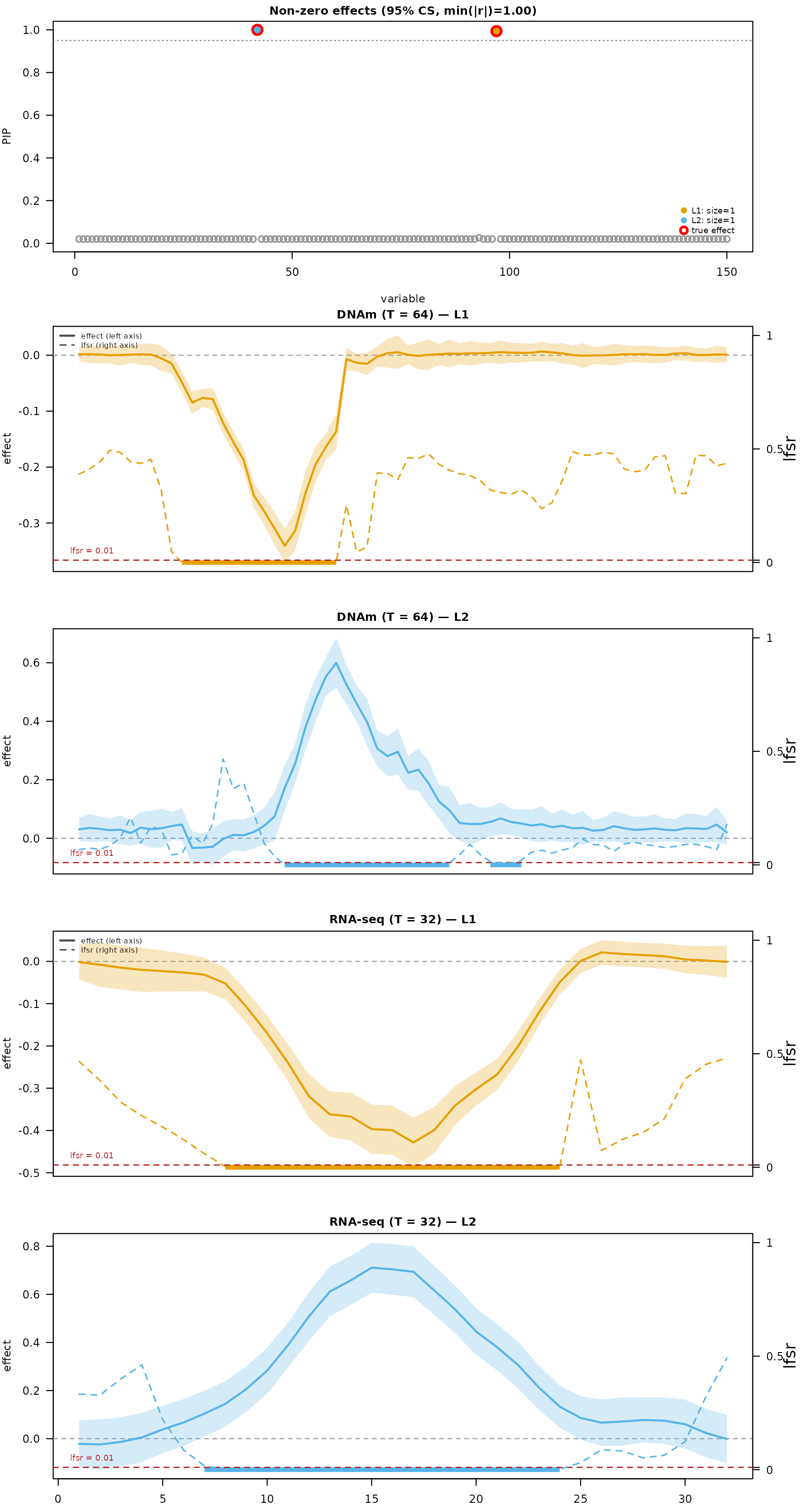

fit$sets$cs
#> $L1
#> [1] 97
#> 
#> $L2
#> [1] 42

coef(fit) returns a list of length M. Element m is an L x T_m matrix containing the per-effect curve for outcome m.

B_hat <- coef(fit)
sapply(B_hat, dim)
#>      [,1] [,2]
#> [1,]    5    5
#> [2,]   64   32

mf_summarize_effects(fit) returns a tidy data frame of the per-(CS, outcome) credibly-non-zero windows (start, end, n_positions), derived from the credible bands of the picked smoother. Useful when you want a tabular handle on which positions each CS lights up at, separately from the plot.

mf_summarize_effects(fit_s)
#>   cs_index outcome start end n_positions
#> 1        1       1    11  26          16
#> 2        2       1    19  37          19
#> 3        2       1    41  44           4
#> 4        1       2     8  24          17
#> 5        2       2     7  24          18

Choosing `prior_variance_scope`

"per_outcome" (default; used above): one mixture-of-normals prior shared across every wavelet scale of an outcome. Appropriate when scales are exchangeable a priori, and roughly S_m-fold cheaper per IBSS iter (one mixsqp call per outcome instead of one per (outcome, scale)).
"per_scale": one mixture per (outcome, scale), letting different scales adapt independently. More flexible at the cost of an S_m-fold larger M-step; useful when shape varies systematically with scale.

Switch between them by changing one argument; the rest of the API and the fit object structure are identical.

Wavelet-domain preprocessing

Three arguments control preprocessing of the per-outcome wavelet matrix before the IBSS loop:

wavelet_magnitude_cutoff (default 0): wavelet columns with median(|column|) <= wavelet_magnitude_cutoff are masked, contributing (Bhat = 0, Shat = 1) to the SER step. Use a small positive value when the response has sparse non-zero entries (e.g., ATAC-seq read pileups).
wavelet_standardize (default TRUE): centers and scales each packed wavelet coefficient column before IBSS. This is a linear, invertible rescaling; fitted values and coefficients are mapped back to the original response scale.
wavelet_qnorm (default FALSE): applies a column-wise rank-normal transform to the wavelet matrix so each wavelet position has marginal N(0, 1) across samples by construction. Useful when the per-outcome residuals are heavy-tailed (read counts, sparse pileups). The transform is non-linear, so coef(fit) curves recover shape and CS membership but not amplitude on the raw Y scale.

wavelet_magnitude_cutoff also routes through mf_adjust_for_covariates(). The qnorm and wavelet-standardize options are fine-mapping preprocessing choices.

When to reach for mfSuSiE over fSuSiE plus colocalization

Use mfsusie() when (i) a variable plausibly affects multiple distinct phenotypes (different tissues, different molecular layers); (ii) the phenotypes have heterogeneous shapes, since mfSuSiE does not require a shared T (some scalar, some functional, some at different sampling resolutions are fine in the same fit); (iii) a single credible-set list combining all the evidence is preferable to a post-hoc colocalization across separate fsusie fits.

Multi-trait data with missing samples

Multi-tissue and multi-cell-type studies often leave some samples unprofiled for some outcomes. Set the corresponding rows of Y[[m]] to NA before calling mfsusie(); the package restricts every regression and variance update to the observed rows for that outcome. Both wavelet_qnorm = FALSE (default) and wavelet_qnorm = TRUE handle missing rows correctly.

set.seed(42)
n <- 80; p <- 60; T_m <- 8; M <- 3
X_miss <- matrix(rbinom(n * p, 2, 0.3), n, p)
X_miss <- scale(X_miss)

# Plant one causal SNP shared across all three traits.
causal_j <- 5L
signal <- as.numeric(X_miss[, causal_j]) * 2
Y_miss <- lapply(seq_len(M), function(m)
  matrix(signal, n, T_m) + matrix(rnorm(n * T_m, sd = 0.5), n, T_m))

# Trait 2 is missing 20 % of rows; trait 3 is missing 30 %.
Y_miss[[2]][sample(n, 16), ] <- NA
Y_miss[[3]][sample(n, 24), ] <- NA

# Per-trait observed sample sizes after masking.
sapply(Y_miss, function(y) sum(complete.cases(y)))
#> [1] 80 64 56

`wavelet_qnorm = FALSE`

t_noq <- system.time(
  fit_noq <- mfsusie(X_miss, Y_miss,
                     wavelet_qnorm = FALSE)
)
#> iter          ELBO       delta   sigma2      mem      V  extras
#>    1    -2181.4266           -   [0.987, 0.997, 1.000]   0.16 GB  [1.20e-01, 0 x 4]  pi_null=[0.87, 1.00]
#> iter   2: max|d(alpha,PIP)|=2.71e-36, V=[1.19e-01, 0 x 4] -- converged (alpha_pip_fixed_point) [mem: 0.16 GB]
#> [L_greedy] 1 round, greedy_lbf_cutoff=0.100, final L=5
#> round  L     min(lbf)   action
#> 1      5     0.000      saturated
cat(sprintf("Runtime: %.1f s   niter: %d   CS: %d\n",
            t_noq["elapsed"], fit_noq$niter, length(fit_noq$sets$cs)))
#> Runtime: 0.7 s   niter: 2   CS: 1
fit_noq$pip[causal_j]                    # causal PIP
#> [1] 1

`wavelet_qnorm = TRUE`

t_q <- system.time(
  fit_q <- mfsusie(X_miss, Y_miss,
                   wavelet_qnorm = TRUE)
)
#> iter          ELBO       delta   sigma2      mem      V  extras
#>    1    -2091.2739           -   [0.987, 0.994, 0.997]   0.16 GB  [5.28e-02, 0 x 4]  pi_null=[0.87, 1.00]
#> iter   2: max|d(alpha,PIP)|=2.22e-16, V=[5.15e-02, 0 x 4] -- converged (alpha_pip_fixed_point) [mem: 0.16 GB]
#> [L_greedy] 1 round, greedy_lbf_cutoff=0.100, final L=5
#> round  L     min(lbf)   action
#> 1      5     0.000      saturated
cat(sprintf("Runtime: %.1f s   niter: %d   CS: %d\n",
            t_q["elapsed"], fit_q$niter, length(fit_q$sets$cs)))
#> Runtime: 0.7 s   niter: 2   CS: 1
fit_q$pip[causal_j]
#> [1] 1

Runtime summary

data.frame(
  path    = c("qnorm=FALSE", "qnorm=TRUE"),
  runtime = c(t_noq["elapsed"], t_q["elapsed"]),
  niter   = c(fit_noq$niter,    fit_q$niter),
  n_cs    = c(length(fit_noq$sets$cs), length(fit_q$sets$cs)),
  causal_pip = c(fit_noq$pip[causal_j], fit_q$pip[causal_j])
)
#>          path runtime niter n_cs causal_pip
#> 1 qnorm=FALSE   0.712     2    1          1
#> 2  qnorm=TRUE   0.702     2    1          1

Session info

This is the version of R and the packages that were used to generate these results.

sessionInfo()
#> R version 4.4.3 (2025-02-28)
#> Platform: x86_64-conda-linux-gnu
#> Running under: Ubuntu 24.04.4 LTS
#> 
#> Matrix products: default
#> BLAS/LAPACK: /home/runner/work/mfsusieR/mfsusieR/.pixi/envs/r44/lib/libopenblasp-r0.3.32.so;  LAPACK version 3.12.0
#> 
#> locale:
#>  [1] LC_CTYPE=C.UTF-8       LC_NUMERIC=C           LC_TIME=C.UTF-8       
#>  [4] LC_COLLATE=C.UTF-8     LC_MONETARY=C.UTF-8    LC_MESSAGES=C.UTF-8   
#>  [7] LC_PAPER=C.UTF-8       LC_NAME=C              LC_ADDRESS=C          
#> [10] LC_TELEPHONE=C         LC_MEASUREMENT=C.UTF-8 LC_IDENTIFICATION=C   
#> 
#> time zone: Etc/UTC
#> tzcode source: system (glibc)
#> 
#> attached base packages:
#> [1] stats     graphics  grDevices utils     datasets  methods   base     
#> 
#> other attached packages:
#> [1] susieR_0.16.1  mfsusieR_0.0.2
#> 
#> loaded via a namespace (and not attached):
#>  [1] sass_0.4.10           generics_0.1.4        ashr_2.2-63          
#>  [4] lattice_0.22-9        digest_0.6.39         magrittr_2.0.5       
#>  [7] RColorBrewer_1.1-3    evaluate_1.0.5        grid_4.4.3           
#> [10] fastmap_1.2.0         plyr_1.8.9            jsonlite_2.0.0       
#> [13] Matrix_1.7-5          reshape_0.8.10        mixsqp_0.3-54        
#> [16] fansi_1.0.7           scales_1.4.0          truncnorm_1.0-9      
#> [19] invgamma_1.2          textshaping_1.0.5     jquerylib_0.1.4      
#> [22] cli_3.6.6             crayon_1.5.3          zigg_0.0.2           
#> [25] rlang_1.2.0           deconvolveR_1.2-1     LaplacesDemon_16.1.8 
#> [28] splines_4.4.3         cachem_1.1.0          yaml_2.3.12          
#> [31] otel_0.2.0            ebnm_1.0-55           tools_4.4.3          
#> [34] SQUAREM_2026.1        parallel_4.4.3        dplyr_1.2.1          
#> [37] wavethresh_4.7.3      ggplot2_4.0.3         Rfast_2.1.5.2        
#> [40] vctrs_0.7.3           R6_2.6.1              matrixStats_1.5.0    
#> [43] lifecycle_1.0.5       fs_2.1.0              htmlwidgets_1.6.4    
#> [46] MASS_7.3-65           trust_0.1-9           ragg_1.5.2           
#> [49] irlba_2.3.7           pkgconfig_2.0.3       desc_1.4.3           
#> [52] RcppParallel_5.1.11-2 pkgdown_2.2.0         bslib_0.10.0         
#> [55] pillar_1.11.1         gtable_0.3.6          glue_1.8.1           
#> [58] Rcpp_1.1.1-1.1        systemfonts_1.3.2     xfun_0.57            
#> [61] tibble_3.3.1          tidyselect_1.2.1      dichromat_2.0-0.1    
#> [64] knitr_1.51            farver_2.1.2          htmltools_0.5.9      
#> [67] rmarkdown_2.31        compiler_4.4.3        S7_0.2.2             
#> [70] horseshoe_0.2.0

Gao Wang, Anjing Liu and William Denault