Why functional fine-mapping
Gao Wang, Anjing Liu and William Denault
Source:vignettes/fsusie_why_functional.Rmd
fsusie_why_functional.RmdThree common alternatives for fine-mapping a functional response all lose information relative to fSuSiE: per-position SuSiE, top-PC SuSiE, and naive multivariate SuSiE. This vignette runs the same simulation that ships with the broader SuSiE-suite diagnostics and shows the four methods side by side. The canonical setup is a single causal SNP whose effect spans 88 out of 128 positions; we report PIPs and recovered effect curves for each method.
Simulation
library(mfsusieR)
library(susieR)
set.seed(1)
data(N3finemapping)
X_full <- N3finemapping$X[seq_len(100), ]
T_m    <- 128L

effect <- 1.2 * cos(seq_len(T_m) / T_m * 3 * pi)
effect[effect < 0] <- 0
effect[seq_len(40)] <- 0     # zero on positions 1..40

true_pos <- 700L
y <- matrix(0, 100L, T_m)
for (i in seq_len(100L)) {
  y[i, ] <- X_full[i, true_pos] * effect + rnorm(T_m)
}
plot(effect, pch = 19, xlab = "position", ylab = "true effect")
Method 1: Per-position SuSiE
For each affected position run susie(X, y[, t], L = 1)
and collect the credible sets. Two failure modes appear: (i) SuSiE
returns no credible set at most affected positions; (ii) when it does
return a CS, the lead variant is inconsistent across nearby
positions.
affected_pos <- which(effect > 0)
susie_est <- vector("list", length(affected_pos))
for (k in seq_along(affected_pos)) {
  susie_est[[k]] <- susie(X, y[, affected_pos[k]], L = 1L)$sets
}
n_cs_per_pos <- vapply(susie_est, function(s) length(s$cs), integer(1L))
table(n_cs_per_pos)
#> n_cs_per_pos
#>  0  1
#> 36  6
Most positions (the 0 column above) yield no CS at all.
Compare positions 88 and 91 to see the second failure: both positions
carry similar effect amplitude, but the per-position SuSiE fits land on
different lead variants, so reasoning about “the causal SNP” from
per-position fits is not straightforward.
illustrate_pos <- function(t) {
  sf <- susie(X, y[, t], L = 1L)
  list(t = t, pip = sf$pip, cs = sf$sets$cs)
}
ill <- list(illustrate_pos(88L), illustrate_pos(91L))

par(mfrow = c(2L, 2L), mar = c(3.5, 4, 2.5, 1))
# Top row: effect curve with the highlighted position.
for (i in seq_along(ill)) {
  plot(effect, pch = 20L, col = "grey60", cex = 0.7,
       xlab = "position", ylab = "true effect",
       main = sprintf("Position %d", ill[[i]]$t),
       cex.main = 1.05, font.main = 2L)
  abline(h = 0, lty = 3, col = "grey50")
  points(ill[[i]]$t, effect[ill[[i]]$t], pch = 21L,
         col = "firebrick", bg = "firebrick", cex = 1.4)
}
# Bottom row: per-position SuSiE PIP.
for (i in seq_along(ill)) {
  plot(ill[[i]]$pip, pch = 20L, col = "grey60", cex = 0.7,
       xlab = "SNP", ylab = "PIP", ylim = c(0, 1),
       main = sprintf("Per-position SuSiE PIP at position %d",
                      ill[[i]]$t),
       cex.main = 1.0, font.main = 2L)
  abline(v = true_pos_filt, lty = 2, col = "grey50")
  cs_l1 <- ill[[i]]$cs$L1
  if (!is.null(cs_l1)) {
    points(cs_l1, ill[[i]]$pip[cs_l1], pch = 19L,
           col = "dodgerblue", cex = 1.2)
  }
  points(true_pos_filt, ill[[i]]$pip[true_pos_filt], pch = 21L,
         col = "firebrick", bg = NA, cex = 1.6, lwd = 1.8)
}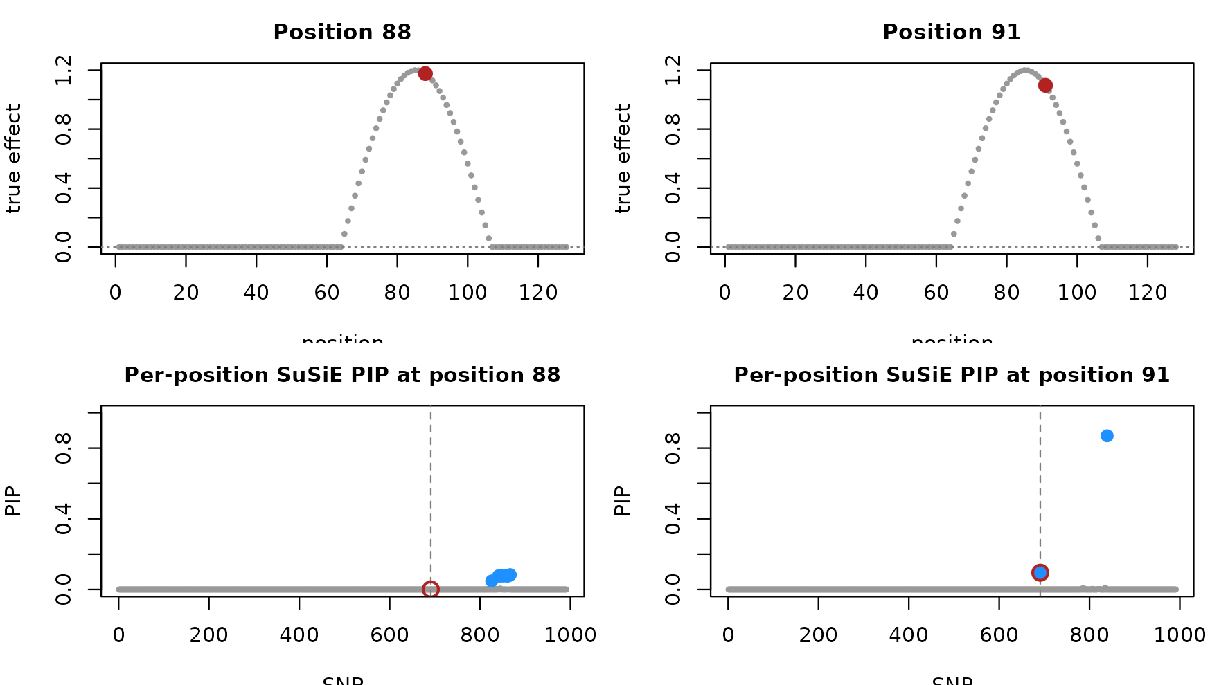
Top row: the per-position truth, with the highlighted position in red. Bottom row: the SuSiE PIP at that position; blue points mark the credible set, red ring marks the true causal SNP. The two positions sit a few CpGs apart yet pick different lead variants, illustrating the per-position-fit incoherence.
Method 2: Top-PC SuSiE for PC = 1..5
Project Y onto its top pc principal
component and fit susie() on each principal component
score:
y_centered <- scale(y, center = TRUE, scale = FALSE)
svd_y <- svd(y_centered)
pc_pip_at_truth <- numeric(5L)
pc_n_cs         <- integer(5L)
for (pc in seq_len(5L)) {
  y_pc <- y_centered %*% svd_y$v[, pc]
  fit_pc <- susie(X, as.numeric(y_pc), L = 1L)
  pc_pip_at_truth[pc] <- fit_pc$pip[true_pos_filt]
  pc_n_cs[pc]         <- length(fit_pc$sets$cs)
}
data.frame(PC = seq_len(5L),
           pip_at_true_snp = pc_pip_at_truth,
           n_cs            = pc_n_cs)
#>   PC pip_at_true_snp n_cs
#> 1  1    1.0000000000    1
#> 2  2    0.0002449867    0
#> 3  3    0.0010065340    0
#> 4  4    0.0000000000    0
#> 5  5    0.0004762581    0
PC 1 captures the trait-driven direction cleanly and SuSiE on the PC 1 score returns a single, high-PIP credible set on the true SNP. That fixes the per-position-SuSiE recall problem: collapsing to one scalar derived from the curve gives a coherent fine-mapping signal. But PCA discards the per-position effect direction. The fit tells us a signal exists at one variant; it does not tell us where on the curve that variant acts. That target information is what fSuSiE preserves and PCA loses.
Method 3: mvSuSiE under default and tuned configurations
mvSuSiE treats Y as a multi-condition
response without a wavelet-basis assumption. Two configurations matter
for this simulation: the default (canonical mixture prior, estimated
residual variance) and the tuned (true outer-product prior, fixed
identity residual variance). The default fails on this data; the tuned
configuration recovers the correct credible set. The PIP-zero failure
mode of the default mvSuSiE on this simulation is the subject of mvsusieR issue
61.
library(mvsusieR)

# Tuned configuration: true outer-product prior + fixed identity
# residual variance. This is the configuration that recovers the
# correct CS.
U_true     <- outer(effect, effect)
prior_true <- create_mixture_prior(
  mixture_prior = list(matrices = list(U_true), weights = 1))
V_true     <- diag(T_m)

fit_mv_tuned <- mvsusie(X, y, L = 1L,
                        prior_variance            = prior_true,
                        residual_variance         = V_true,
                        estimate_residual_variance = FALSE,
                        estimate_prior_variance    = TRUE,
                        max_iter = 100L, verbose = FALSE)
cat("PIP at true SNP (tuned):", fit_mv_tuned$pip[true_pos_filt], "\n")
#> PIP at true SNP (tuned): 1
cat("CS count (tuned):", length(fit_mv_tuned$sets$cs), "\n")
#> CS count (tuned): 1

# Default configuration: canonical mixture prior, estimated
# residual variance. The PIPs collapse to zero on this data
# (mvsusieR issue 61).
prior_canon <- create_mixture_prior(R = T_m)
fit_mv_default <- mvsusie(X, y, L = 1L,
                          prior_variance = prior_canon,
                          max_iter = 100L, verbose = FALSE)
cat("Max PIP (default):", max(fit_mv_default$pip), "\n")
#> Max PIP (default): 0
cat("CS count (default):", length(fit_mv_default$sets$cs), "\n")
#> CS count (default): 0
# Recovered effect curves from both mvSuSiE configurations.
# `coef()` on an mvsusie fit returns a (J + 1) x R matrix; row
# j + 1 is the fitted effect curve of SNP j across positions.
lead_tuned   <- which.max(fit_mv_tuned$pip)
lead_default <- which.max(fit_mv_default$pip)
mv_eff_tuned   <- as.numeric(coef(fit_mv_tuned)[lead_tuned + 1L, ])
mv_eff_default <- as.numeric(coef(fit_mv_default)[lead_default + 1L, ])

par(mfrow = c(1L, 2L), mar = c(4, 4, 2.5, 1))
yrng <- range(c(effect, mv_eff_tuned, mv_eff_default))
plot(effect, pch = 20L, col = "grey30", cex = 0.7, ylim = yrng,
     xlab = "position", ylab = "effect",
     main = "mvSuSiE tuned (truth-informed prior)",
     cex.main = 1.05, font.main = 2L)
abline(h = 0, lty = 3, col = "grey50")
lines(mv_eff_tuned, col = "firebrick", lwd = 2)
legend("topright", legend = c("truth", "mvSuSiE tuned"),
       col = c("grey30", "firebrick"), lwd = c(NA, 2),
       lty = c(NA, 1), pch = c(20, NA), bty = "n", cex = 0.8)

plot(effect, pch = 20L, col = "grey30", cex = 0.7, ylim = yrng,
     xlab = "position", ylab = "effect",
     main = "mvSuSiE default (canonical prior)",
     cex.main = 1.05, font.main = 2L)
abline(h = 0, lty = 3, col = "grey50")
lines(mv_eff_default, col = "firebrick", lwd = 2)
legend("topright", legend = c("truth", "mvSuSiE default"),
       col = c("grey30", "firebrick"), lwd = c(NA, 2),
       lty = c(NA, 1), pch = c(20, NA), bty = "n", cex = 0.8)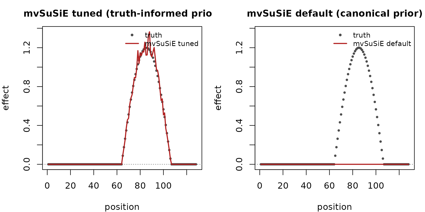
The tuned configuration recovers the effect shape closely. The default configuration’s recovered curve is essentially flat at zero: with no truth-informed prior the canonical mixture cannot distinguish the signal from noise, the PIPs collapse, and the fitted effect carries no information. The signal is recoverable only when the true effect direction is supplied as the prior.
Method 4: fSuSiE
A single fsusie() call recovers the correct credible set
and a smooth recovered effect curve, no truth-informed configuration
required.
fit_f <- fsusie(y, X, verbose = FALSE)
fit_f$sets$cs
#> $L1
#> [1] 691
fit_f$pip[true_pos_filt]
#> [1] 1
The default mfsusie_plot() shows PIPs in the top panel
and the TI-smoothed effect curve with 95% credible band in the bottom
panel. Pass truth = list(effect) to overlay the
per-position truth as dark-grey dots; the true causal SNP is highlighted
on the PIP panel with a red ring and a vertical dashed reference.
fit_f_s <- mf_post_smooth(fit_f)
plot_dims <- mfsusie_plot_dimensions(fit_f_s)
mfsusie_plot(fit_f_s, truth = list(effect))
# Highlight the true causal SNP on the PIP panel.
abline(v = true_pos_filt, lty = 2, col = "firebrick", lwd = 1.2)
points(true_pos_filt, fit_f_s$pip[true_pos_filt], pch = 21L,
       col = "firebrick", bg = NA, cex = 1.6, lwd = 2)
The credible set lands on the true SNP, and the smoothed effect curve tracks the truth across the affected support.
For a publication-style view, build PIP and per-effect panels
directly from fit_f’s posterior fields:
library(ggplot2)
library(cowplot)

ti          <- fit_f_s$smoothed$TI
mean_curve  <- ti$effect_curves[[1L]][[1L]]
band        <- ti$credible_bands[[1L]][[1L]]
df_truth    <- data.frame(x = seq_along(effect),     y = effect)
df_curve    <- data.frame(x = seq_along(mean_curve), y = mean_curve)
df_band     <- data.frame(x  = seq_along(mean_curve),
                          lo = band[, 1L], hi = band[, 2L])

P_effect <- ggplot() +
  geom_ribbon(data = df_band,
              mapping = aes(x = x, ymin = lo, ymax = hi),
              fill = "skyblue", alpha = 0.45) +
  geom_point(data = df_truth, mapping = aes(x = x, y = y),
             color = "grey30", size = 1.2) +
  geom_line(data = df_curve, mapping = aes(x = x, y = y),
            color = "firebrick", linewidth = 1) +
  geom_hline(yintercept = 0, linetype = "dotted", color = "grey50") +
  labs(x = "position", y = "effect",
       title = "fSuSiE recovered effect curve") +
  theme_classic()

df_pip <- data.frame(x = seq_along(fit_f$pip), y = fit_f$pip)
P_pip <- ggplot(df_pip, aes(x = x, y = y)) +
  geom_point(color = "grey60", size = 0.9) +
  geom_point(data = df_pip[true_pos_filt, , drop = FALSE],
             color = "firebrick", size = 2.2) +
  geom_vline(xintercept = true_pos_filt,
             linetype = "dashed", color = "firebrick", alpha = 0.6) +
  ylim(0, 1) +
  labs(x = "SNP", y = "PIP", title = "fSuSiE PIPs") +
  theme_classic()

plot_grid(P_pip, P_effect, nrow = 1L, ncol = 2L,
          rel_widths = c(1, 1.2))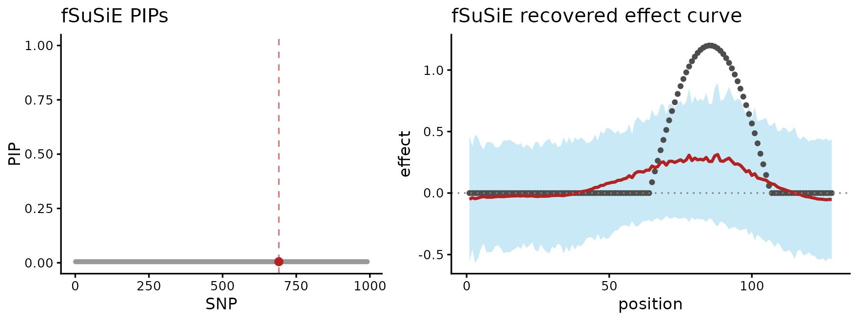
The PIP scatter on the left puts a single point at PIP near 1 on the true causal SNP (red); the effect-curve on the right has the credible band hugging the truth across the affected positions. The shape, the zero-effect prefix on positions 1..40, and the peak around the cosine maximum are all recovered cleanly without any truth-informed prior or pre-specified number of effects.
When to use which tool in the SuSiE suite
Per-position SuSiE is appropriate when only one position is expected to carry signal and that position is known a priori. Top-PC SuSiE is appropriate when the principal-component direction aligns with the variable-driven effect (rare in practice). mvSuSiE is appropriate when the response has a small, fixed number of conditions and a meaningful between- condition covariance prior is available. fSuSiE is appropriate when the response is a smooth function of position and the position grid is power-of-two (or remappable to one), which covers methylation, accessibility, and coverage-style traits.
Session info
This is the version of R and the packages that were used to generate these results.
sessionInfo()
#> R version 4.4.3 (2025-02-28)
#> Platform: x86_64-conda-linux-gnu
#> Running under: Ubuntu 24.04.4 LTS
#>
#> Matrix products: default
#> BLAS/LAPACK: /home/runner/work/mfsusieR/mfsusieR/.pixi/envs/r44/lib/libopenblasp-r0.3.32.so;  LAPACK version 3.12.0
#>
#> locale:
#>  [1] LC_CTYPE=C.UTF-8       LC_NUMERIC=C           LC_TIME=C.UTF-8
#>  [4] LC_COLLATE=C.UTF-8     LC_MONETARY=C.UTF-8    LC_MESSAGES=C.UTF-8
#>  [7] LC_PAPER=C.UTF-8       LC_NAME=C              LC_ADDRESS=C
#> [10] LC_TELEPHONE=C         LC_MEASUREMENT=C.UTF-8 LC_IDENTIFICATION=C
#>
#> time zone: Etc/UTC
#> tzcode source: system (glibc)
#>
#> attached base packages:
#> [1] stats     graphics  grDevices utils     datasets  methods   base
#>
#> other attached packages:
#> [1] cowplot_1.2.0  ggplot2_4.0.3  mvsusieR_0.2.0 mashr_0.2.79   ashr_2.2-63
#> [6] susieR_0.16.1  mfsusieR_0.0.2
#>
#> loaded via a namespace (and not attached):
#>  [1] gtable_0.3.6          xfun_0.57             bslib_0.10.0
#>  [4] htmlwidgets_1.6.4     ggrepel_0.9.8         ebnm_1.0-55
#>  [7] lattice_0.22-9        vctrs_0.7.3           tools_4.4.3
#> [10] generics_0.1.4        parallel_4.4.3        tibble_3.3.1
#> [13] pkgconfig_2.0.3       Matrix_1.7-5          SQUAREM_2026.1
#> [16] RColorBrewer_1.1-3    S7_0.2.2              desc_1.4.3
#> [19] RcppParallel_5.1.11-2 assertthat_0.2.1      lifecycle_1.0.5
#> [22] truncnorm_1.0-9       compiler_4.4.3        farver_2.1.2
#> [25] textshaping_1.0.5     wavethresh_4.7.3      htmltools_0.5.9
#> [28] sass_0.4.10           yaml_2.3.12           pillar_1.11.1
#> [31] pkgdown_2.2.0         crayon_1.5.3          jquerylib_0.1.4
#> [34] MASS_7.3-65           cachem_1.1.0          rmeta_3.0
#> [37] trust_0.1-9           abind_1.4-8           tidyselect_1.2.1
#> [40] digest_0.6.39         mvtnorm_1.3-7         dplyr_1.2.1
#> [43] LaplacesDemon_16.1.8  labeling_0.4.3        splines_4.4.3
#> [46] fastmap_1.2.0         grid_4.4.3            cli_3.6.6
#> [49] invgamma_1.2          magrittr_2.0.5        dichromat_2.0-0.1
#> [52] Rfast_2.1.5.2         withr_3.0.2           scales_1.4.0
#> [55] horseshoe_0.2.0       rmarkdown_2.31        matrixStats_1.5.0
#> [58] otel_0.2.0            deconvolveR_1.2-1     ragg_1.5.2
#> [61] evaluate_1.0.5        knitr_1.51            irlba_2.3.7
#> [64] rlang_1.2.0           zigg_0.0.2            Rcpp_1.1.1-1.1
#> [67] mixsqp_0.3-54         glue_1.8.1            reshape_0.8.10
#> [70] jsonlite_2.0.0        R6_2.6.1              plyr_1.8.9
#> [73] systemfonts_1.3.2     fs_2.1.0