Smoothing effect curves and credible bands
Gao Wang, Anjing Liu and William Denault
Source:vignettes/post_processing.Rmd
post_processing.RmdWhy post-process
mfsusie() and fsusie() fit the model in the
wavelet domain. The per-effect posterior is summarized by
coef(fit), which inverts the wavelet representation back to
position space. The raw inverse curve is correct but visually wiggly:
small fine-scale wavelet coefficients contribute pointwise noise that
obscures the underlying shape, and the fit returns no pointwise credible
band by default.
The post-processor mf_post_smooth(fit, method = ...)
runs the chosen smoother on the per-effect wavelet posterior mean and
stores the result on the fit at fit$smoothed[[method]]. The
slot carries:
-
fit$smoothed[[method]]$effect_curves[[m]][[l]]: smoothed position-space curve for outcomem, effectl. -
fit$smoothed[[method]]$credible_bands[[m]][[l]]:T_basis x 2matrix[lower, upper]. -
fit$smoothed$HMM$lfsr_curves[[m]][[l]]: per-position local false sign rate (HMM only).
The fit accumulates per-method results: every call to
mf_post_smooth(fit, method = ...) adds (or, with
overwrite_previous = TRUE, replaces) one entry in
fit$smoothed. The raw inverse-DWT curves remain accessible
via coef(fit); pass
coef(fit, smooth_method = "TI") to get the TI-smoothed
curves on the same list[M] of L x T_basis
matrix shape.
mfsusie_plot() reads from fit$smoothed and
picks a smoother in the priority order
HMM > TI > smash > ash > scalewise when the
user does not name one explicitly. When more than one smoother has been
applied, the plot emits a hint listing the alternatives so the user can
compare. After method = "HMM" smoothing the per-position
lfsr curves are also overlaid on a secondary axis with a threshold line
at lfsr_threshold = 0.05. Affected regions (where each CS’s
credible band excludes zero) are marked with thick bars at the bottom of
each effect panel.
A small example
Simulate one functional outcome with a smooth bell-shaped effect at each of two causal variables:
data(N3finemapping)
X <- N3finemapping$X[, seq_len(150)]
n <- nrow(X); p <- ncol(X); T_m <- 64

positions <- seq_len(T_m)
shape <- exp(-((positions - T_m / 2)^2) / (2 * (T_m / 8)^2))
beta <- matrix(0, p, T_m)
beta[42, ] <-  1.5 * shape
beta[97, ] <- -1.0 * shape
Y <- X %*% beta + matrix(rnorm(n * T_m, sd = 0.5), n)

fit <- fsusie(Y, X, pos = positions)
#> iter          ELBO       delta   sigma2      mem      V  extras
#>    1   -51276.3615           -   [0.998, 0.999, 1.000]   0.17 GB  [4.03e-02, 9.79e-03, 0 x 3]  pi_null=[0.85, 1.00]
#> iter   2: max|d(alpha,PIP)|=9.99e-16, V=[4.05e-02, 9.75e-03, 0 x 3] -- converged (alpha_pip_fixed_point) [mem: 0.17 GB]
#> [L_greedy] 1 round, greedy_lbf_cutoff=0.100, final L=5
#> round  L     min(lbf)   action
#> 1      5     0.000      saturated
Before smoothing
mfsusie_plot() on the unsmoothed fit shows curves
recovered from coef() (raw inverse DWT). The curves track
the true bell shape, but fine wavelet scales contribute high-frequency
noise, and the fit returns no credible bands by default.
plot_dims_b <- mfsusie_plot_dimensions(fit)
mfsusie_plot(fit)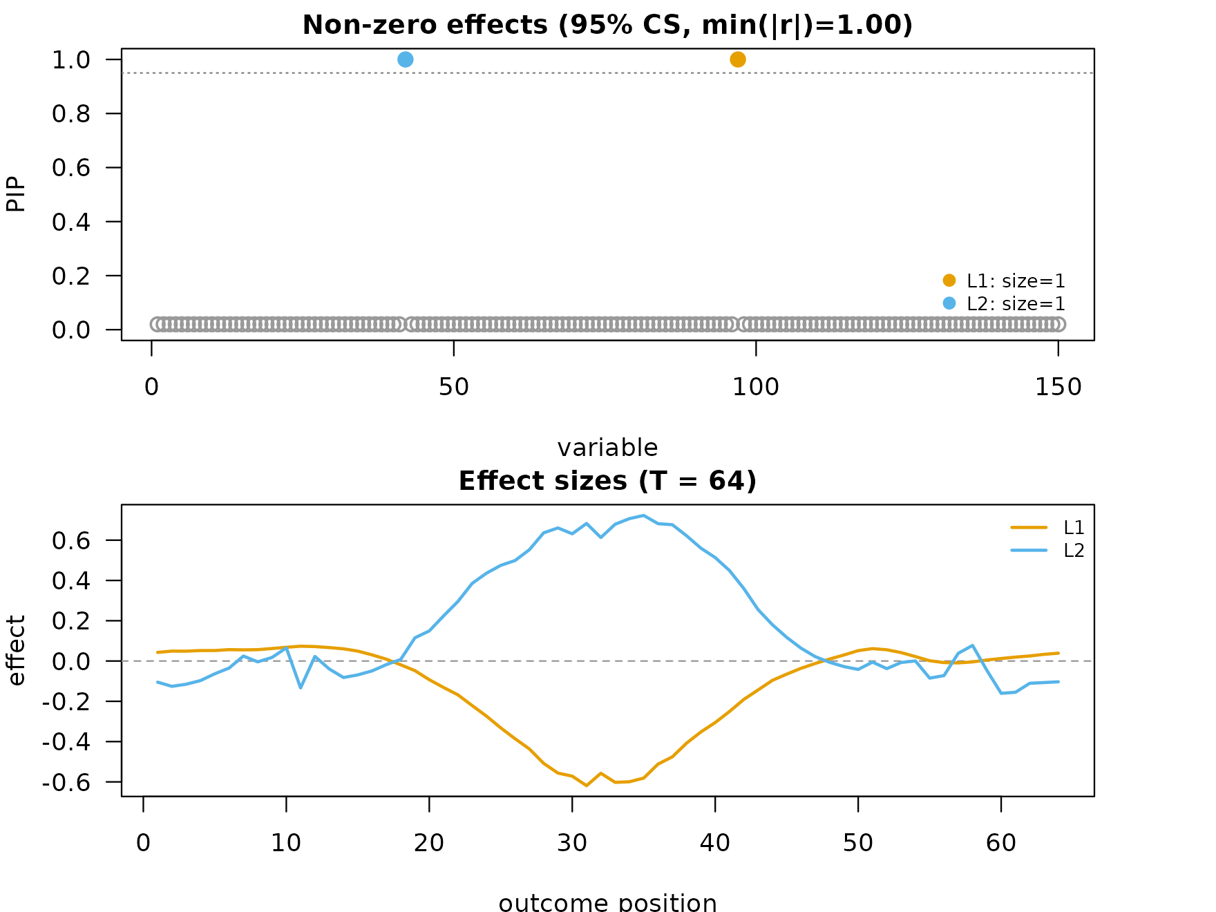
After smoothing
fit_s <- mf_post_smooth(fit)            # default method = "TI"
names(fit_s$smoothed)                   # which smoothings are on the fit
#> [1] "TI"
The same plot call now reads fit_s$smoothed$TI and adds
95% pointwise credible bands as transparent ribbons:
plot_dims_a <- mfsusie_plot_dimensions(fit_s)
mfsusie_plot(fit_s)
The shape is preserved, high-frequency noise is suppressed, and the ribbon marks the positions where the band excludes zero.
Stacking multiple smoothers on one fit
Every call to mf_post_smooth(fit, method = ...) adds an
entry to fit$smoothed rather than overwriting the previous
result. Comparing methods is a few lines:
fit_s <- mf_post_smooth(fit_s, method = "HMM")
fit_s <- mf_post_smooth(fit_s, method = "scalewise")
names(fit_s$smoothed)
#> [1] "TI"        "HMM"       "scalewise"
coef() exposes the same multi-method state via the
smooth_method argument:
str(coef(fit_s),                          max.level = 1L)  # raw inverse DWT
#> List of 1
#>  $ : num [1:5, 1:64] 0.0182 -0.0424 0 0 0 ...
str(coef(fit_s, smooth_method = "TI"),    max.level = 1L)
#> List of 1
#>  $ : num [1:5, 1:64] 0.0061 0.018 0.0112 0.0112 0.0112 ...
#>  - attr(*, "smooth_method")= chr "TI"
str(coef(fit_s, smooth_method = "HMM"),   max.level = 1L)
#> List of 1
#>  $ : num [1:5, 1:64] -5.27e-08 5.80e-07 -1.41e-03 -1.41e-03 -1.41e-03 ...
#>  - attr(*, "smooth_method")= chr "HMM"
Because coef(fit) defaults to the raw inverse DWT,
smoothing is always an explicit opt-in. Pass
smooth_method = "<name>" when you want the
post-processed curves.
Choosing a smoother
mf_post_smooth(method = ...) supports four methods:
-
"TI"(default): translation-invariant wavelet denoising via cycle spinning. Best when the per-position band is the visual focus. -
"scalewise": per-scale soft-thresholding of the wavelet posterior mean atthreshold_factor * sd_s * sqrt(2 log T), followed by inverse DWT. Cheapest, no extra dependencies. Lowers fine-scale jitter while preserving the overall shape. -
"HMM": hidden Markov model on per-position regression estimates withashrmixture refinement. Adds a per-position local false sign rate (lfsr_curves);mfsusie_plot()overlays it on a secondary axis with the threshold line. -
"smash":smashr::smash.gausempirical-Bayes wavelet shrinkage on the per-position regression estimate. Requires thesmashrpackage (Suggests). -
"ash": cycle-spinning + per-coefficientashr::ashon the wavelet decomposition of the per-position estimate, using the per-position OLS Shat as the noise level. Same niche as"smash"but does not require thesmashrpackage.
All five smoothers can coexist on the same fit.
mfsusie_plot() picks one by priority (HMM > TI >
smash > ash > scalewise) and emits a hint listing the others; pass
smooth_method = "<name>" to plot a specific one.
fit_scalewise <- mf_post_smooth(fit, method = "scalewise",
                                threshold_factor = 0.5)
plot_dims_sc <- mfsusie_plot_dimensions(fit_scalewise,
                                        smooth_method = "scalewise")
mfsusie_plot(fit_scalewise, smooth_method = "scalewise")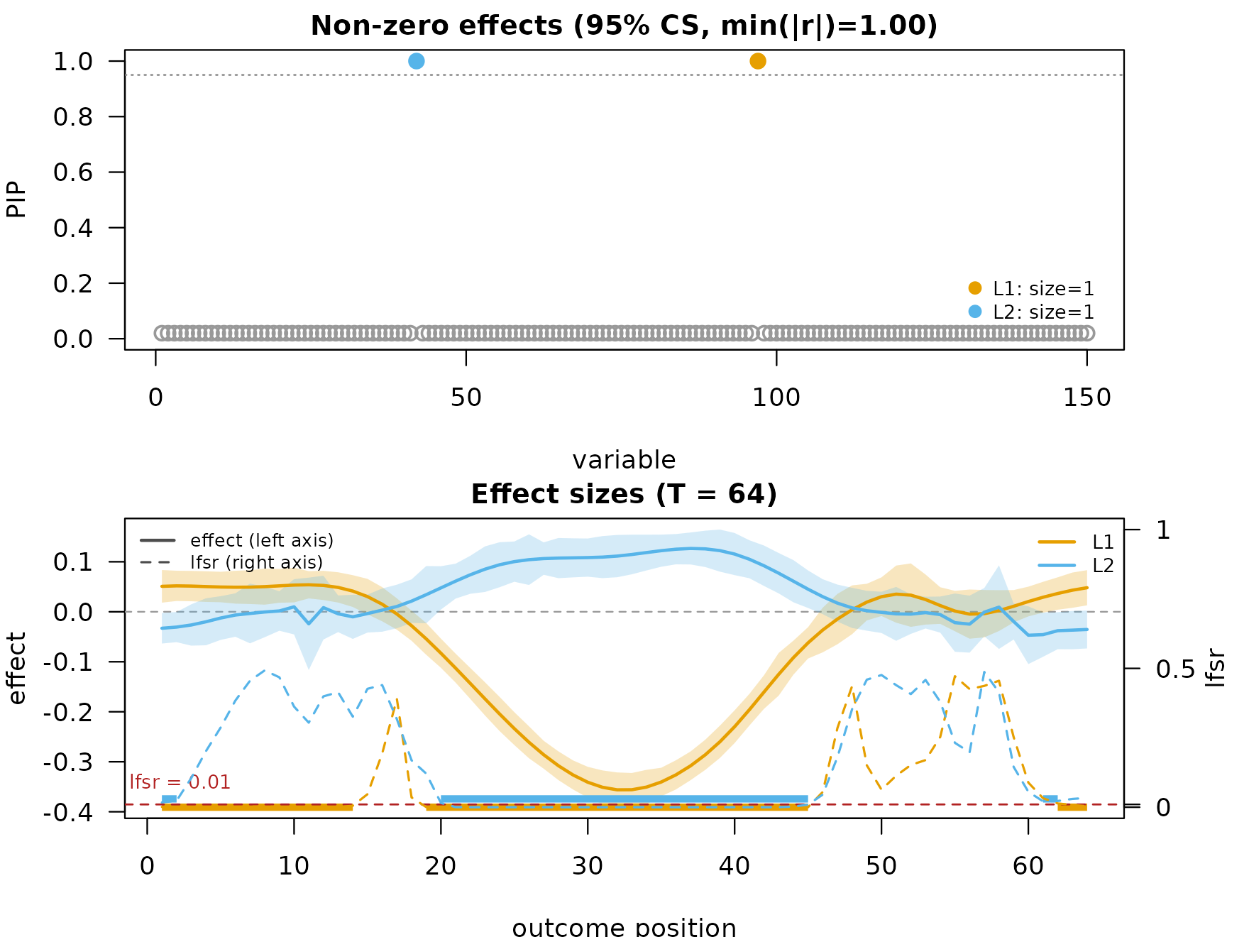
fit_hmm <- mf_post_smooth(fit, method = "HMM")
plot_dims_hm <- mfsusie_plot_dimensions(fit_hmm)
mfsusie_plot(fit_hmm) # picks HMM (the only smoother on the fit)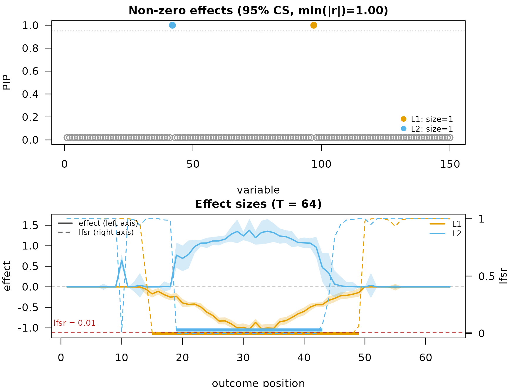
fit_smash <- mf_post_smooth(fit, method = "smash")
plot_dims_sm <- mfsusie_plot_dimensions(fit_smash)
mfsusie_plot(fit_smash)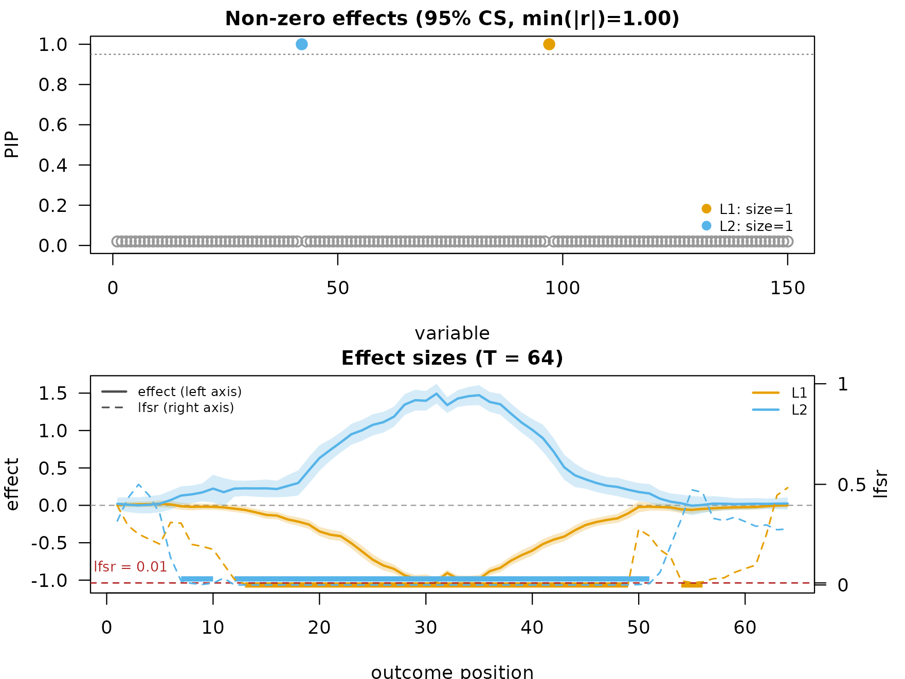
When several smoothers are stacked, plotting picks the highest-priority one and lists the others as a hint:
fit_multi <- mf_post_smooth(fit)
fit_multi <- mf_post_smooth(fit_multi, method = "HMM")
fit_multi <- mf_post_smooth(fit_multi, method = "scalewise")
plot_dims_ml <- mfsusie_plot_dimensions(fit_multi)
#> HINT: Plotting smoothing 'HMM'. Other smoothings on this fit: 'TI', 'scalewise'. Pass `smooth_method = '<name>'` to plot a different one.
mfsusie_plot(fit_multi)                              # picks HMM; hint prints
#> HINT: Plotting smoothing 'HMM'. Other smoothings on this fit: 'TI', 'scalewise'. Pass `smooth_method = '<name>'` to plot a different one.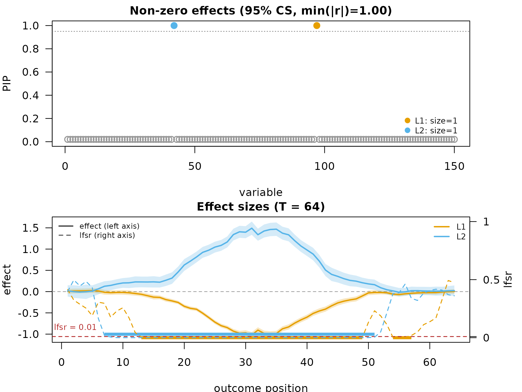
mfsusie_plot(fit_multi, smooth_method = "TI") # plot TI directly
Per-variant lfsr (clfsr) and the smashr-free
smoother
Three additions complement the four core smoothers above. Each is a one-line opt-in.
clfsr_curves: per-variant lfsr
Every smoother also writes a clfsr_curves[[m]][[l]] slot
of shape p x T_basis[m]: the per-variant local false sign
rate derived from the SuSiE posterior moments
pnorm(-|mu[l, m, j, t]| / sd[l, m, j, t]). This is the
per-variant view that the alpha-aggregated lfsr_curves
summary hides. It is useful when you want to ask “is variant
j credibly nonzero at position t?” rather than
“is the credible set credibly nonzero at position t?”.
The plot has a toggle that swaps the alpha-aggregated lfsr overlay
for the alpha-aggregated clfsr curve:
plot_dims_cl <- mfsusie_plot_dimensions(fit_s)
#> HINT: Plotting smoothing 'HMM'. Other smoothings on this fit: 'TI', 'scalewise'. Pass `smooth_method = '<name>'` to plot a different one.
mfsusie_plot(fit_s, lfsr_source = "clfsr")
#> HINT: Plotting smoothing 'HMM'. Other smoothings on this fit: 'TI', 'scalewise'. Pass `smooth_method = '<name>'` to plot a different one.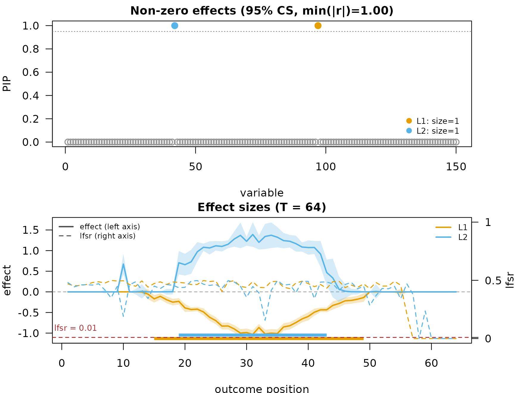
method = "ash" for installs without
smashr
mf_post_smooth(fit, method = "ash") runs the same
cycle-spinning + ash kernel that smash_lw uses upstream,
with the per-position OLS standard error as the noise level. It needs
only ashr and wavethresh (both already in
Imports).
fit_ash <- mf_post_smooth(fit, method = "ash")
str(fit_ash$smoothed$ash$effect_curves[[1]][[1]])
#>  num [1:64] 0.0118 0.0131 0.0131 0.0133 0.0114 ...
Tuning the underlying shrinkage tool via ...
mf_post_smooth(method = "TI" | "HMM" | "ash", ...)
forwards extra arguments to ashr::ash;
method = "smash" forwards to
smashr::smash.gaus. The most useful knob is
nullweight, which controls how aggressively the null
component is preferred:
fit_strong <- mf_post_smooth(fit, method = "ash", nullweight = 300)Higher nullweight shrinks effects toward zero more
aggressively and is the right choice on noisy fixtures with weak
signal.
Per-CS lfsr bubble grid
mfsusie_plot_lfsr(fit) draws a per-CS-by-position bubble
grid: one row per credible set, one dot per position, dot size
-log10(lfsr), colored by the CS when the position clears
lfsr_threshold. The same lfsr_source toggle as
mfsusie_plot() selects which lfsr to show.
fit_hmm <- mf_post_smooth(fit, method = "HMM")
plot_dims_lfsr <- mfsusie_plot_lfsr_dimensions(fit_hmm)
mfsusie_plot_lfsr(fit_hmm, lfsr_source = "lfsr")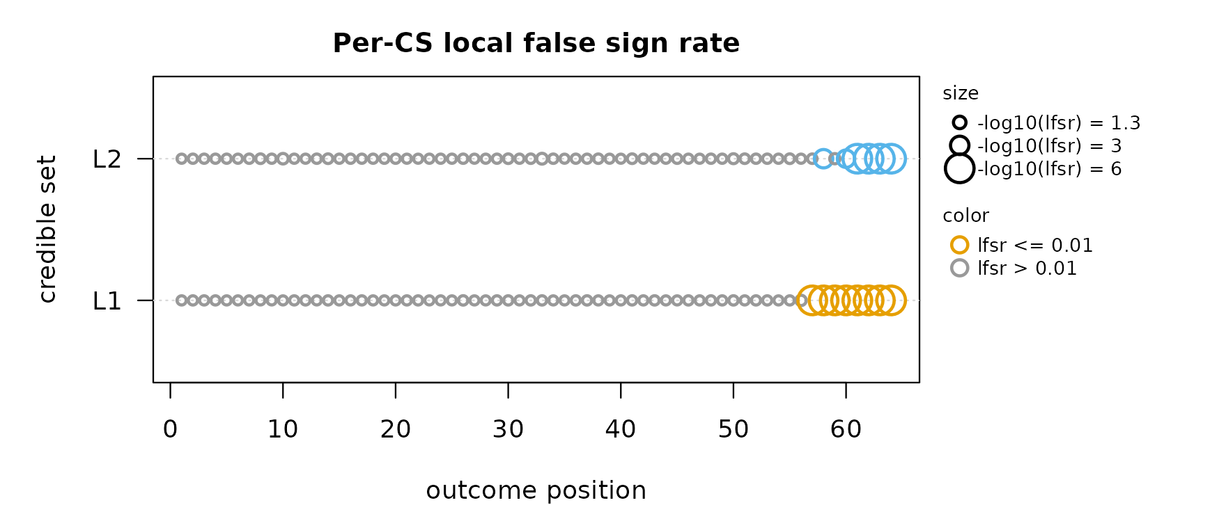
lfsr_source = "lfsr" is computed from the SuSiE
posterior moments, so it works on a fit that has not been post-smoothed
(no need for method = "HMM" first); it just needs the
bubble-grid layout, which the function still provides.
Multi-outcome usage
mf_post_smooth() works on mfsusie() fits
the same way; the chosen entry of fit$smoothed[[method]]
carries effect_curves[[m]] and
credible_bands[[m]] for every functional outcome. Scalar
outcomes (T_m = 1) are passed through (no smoothing needed)
and get a band derived from the wavelet posterior SD.
# Two functional outcomes at different sampling resolutions
# (T = 64 and T = 32). Same two causal variables, different
# per-outcome bell shapes.
T_per <- c(64L, 32L)
shape64 <- exp(-((seq_len(64) - 32)^2) / (2 * 8^2))
shape32 <- exp(-((seq_len(32) - 16)^2) / (2 * 4^2))
beta1 <- matrix(0, p, 64L); beta1[42, ] <- 1.5 * shape64
                            beta1[97, ] <- -1.0 * shape64
beta2 <- matrix(0, p, 32L); beta2[42, ] <- 1.0 * shape32
                            beta2[97, ] <- -0.6 * shape32
Y_list <- list(
  X %*% beta1 + matrix(rnorm(n * 64, sd = 0.5), n),
  X %*% beta2 + matrix(rnorm(n * 32, sd = 0.4), n)
)

fit_m   <- mfsusie(X, Y_list)
#> iter          ELBO       delta   sigma2      mem      V  extras
#>    1   -76876.7213           -   [0.998, 0.999, 1.000]   0.18 GB  [3.62e-02, 8.62e-03, 0 x 3]  pi_null=[0.86, 1.00]
#> iter   2: max|d(alpha,PIP)|=1.12e-01, V=[3.66e-02, 8.71e-03, 2.52e-04, 0 x 2] [mem: 0.18 GB]
#> iter   3: max|d(alpha,PIP)|=4.62e-01, V=[3.66e-02, 8.71e-03, 7.15e-04, 0 x 2] [mem: 0.18 GB]
#> iter   4: max|d(alpha,PIP)|=4.64e-01, V=[3.65e-02, 8.71e-03, 7.19e-04, 0 x 2] [mem: 0.18 GB]
#> iter   5: max|d(alpha,PIP)|=1.50e-05, V=[3.65e-02, 8.71e-03, 7.19e-04, 0 x 2] -- converged (alpha_pip_fixed_point) [mem: 0.18 GB]
#> [L_greedy] 1 round, greedy_lbf_cutoff=0.100, final L=5
#> round  L     min(lbf)   action
#> 1      5     0.000      saturated
fit_m_s <- mf_post_smooth(fit_m)
plot_dims_ms <- mfsusie_plot_dimensions(fit_m_s)
mfsusie_plot(fit_m_s)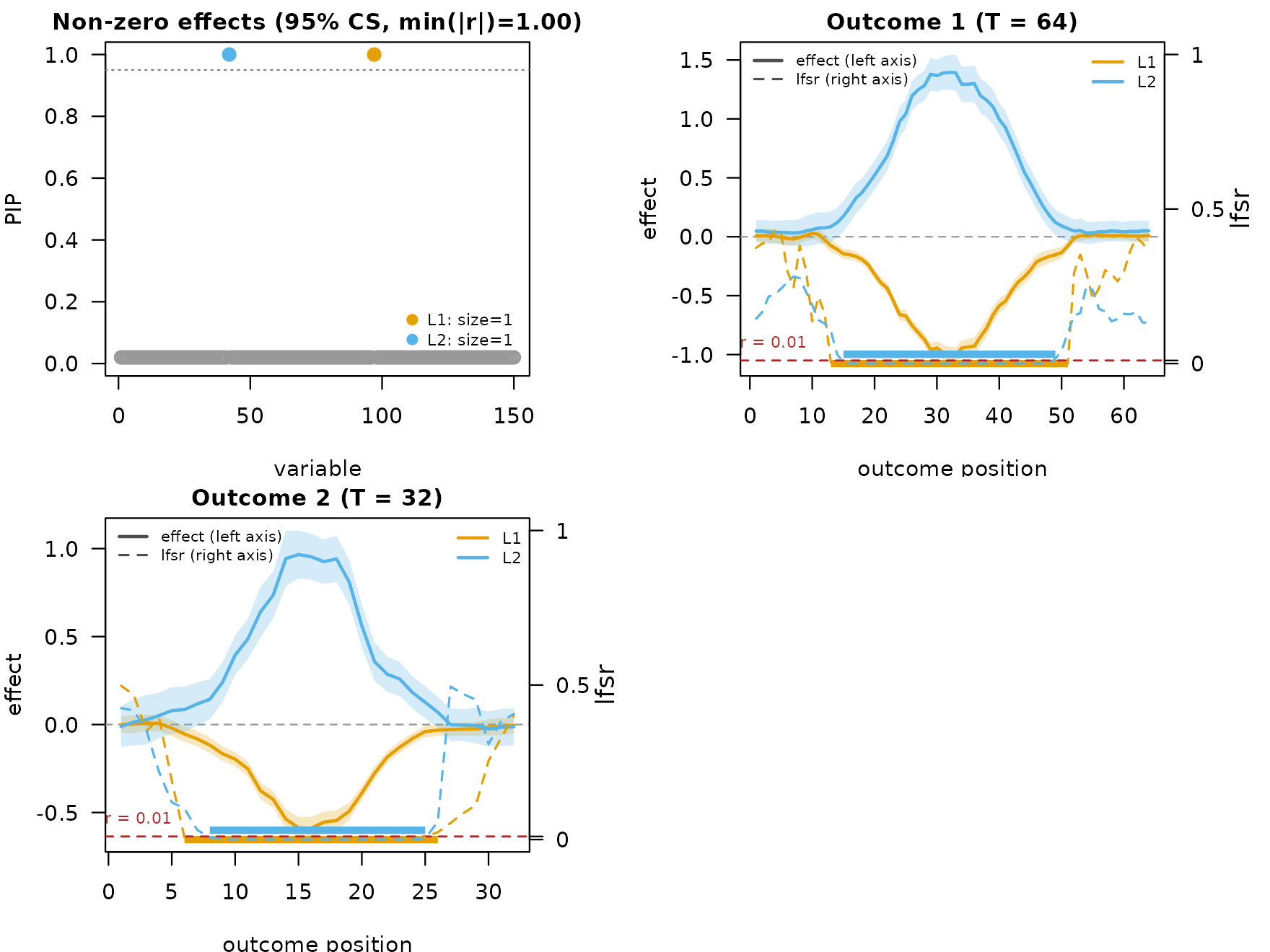
Method
Each method takes the per-effect wavelet-domain posterior
(mean_w, var_w) = (alpha[l, ] %*% mu[[l]][[m]], alpha[l, ] %*% mu2[[l]][[m]] - mean_w^2)
and produces a smoothed position-space curve plus a pointwise credible
band:
-
"TI": cycle spinning. At every shift, run a stationary DWT with squared filter coefficients to compute pointwise variance, apply ash to the wavelet coefficients per scale, and average the inverse reconstructions across shifts. Credible bands come from the average-of-basis variance kernel. -
"scalewise": soft-thresholdmean_w[scale_index[[s]]]per wavelet scalesatthreshold_factor * sd_s * sqrt(2 log T), then invert viamf_invert_dwt(). The pointwise variance is the position-space variance from the wavelet posterior:Var(pos[t]) = sum_k W^T_{tk}^2 * var_w[k]whereW^Tis the inverse-DWT matrix. The band is `mean_pos +/- z(level)- sqrt(Var(pos))`.
-
"HMM": discrete-state hidden Markov model on per-position regression estimates with hub-and-spoke transitions and ash refinement at each EM iteration. The smoothed curve is the posterior mean. The pointwise SD comes from the law of total variance over the HMM state mixture: `Var(pos[t]) = sum_k prob[t, k] * (sd_kt^2 + mean_kt^2)- (sum_k prob[t, k] * mean_kt)^2
, whereprob[t, k]is the forward-backward state probability and(mean_kt, sd_kt)are the per-state ash posterior moments. Band asmean_pos +/- z(level) * sqrt(Var(pos))`.
- (sum_k prob[t, k] * mean_kt)^2
-
"smash":smashr::smash.gausempirical-Bayes wavelet shrinkage on the per-position regression estimate of the effect against the lead variable. The credible band usessmash’spost.var = TRUEposterior variance.
Session info
This is the version of R and the packages that were used to generate these results.
sessionInfo()
#> R version 4.4.3 (2025-02-28)
#> Platform: x86_64-conda-linux-gnu
#> Running under: Ubuntu 24.04.4 LTS
#>
#> Matrix products: default
#> BLAS/LAPACK: /home/runner/work/mfsusieR/mfsusieR/.pixi/envs/r44/lib/libopenblasp-r0.3.32.so;  LAPACK version 3.12.0
#>
#> locale:
#>  [1] LC_CTYPE=C.UTF-8       LC_NUMERIC=C           LC_TIME=C.UTF-8
#>  [4] LC_COLLATE=C.UTF-8     LC_MONETARY=C.UTF-8    LC_MESSAGES=C.UTF-8
#>  [7] LC_PAPER=C.UTF-8       LC_NAME=C              LC_ADDRESS=C
#> [10] LC_TELEPHONE=C         LC_MEASUREMENT=C.UTF-8 LC_IDENTIFICATION=C
#>
#> time zone: Etc/UTC
#> tzcode source: system (glibc)
#>
#> attached base packages:
#> [1] stats     graphics  grDevices utils     datasets  methods   base
#>
#> other attached packages:
#> [1] susieR_0.16.1  mfsusieR_0.0.2
#>
#> loaded via a namespace (and not attached):
#>  [1] gtable_0.3.6          xfun_0.57             bslib_0.10.0
#>  [4] ggplot2_4.0.3         smashr_1.2-7          htmlwidgets_1.6.4
#>  [7] caTools_1.18.3        ebnm_1.0-55           lattice_0.22-9
#> [10] vctrs_0.7.3           tools_4.4.3           bitops_1.0-9
#> [13] generics_0.1.4        parallel_4.4.3        tibble_3.3.1
#> [16] pkgconfig_2.0.3       Matrix_1.7-5          data.table_1.17.8
#> [19] SQUAREM_2026.1        RColorBrewer_1.1-3    S7_0.2.2
#> [22] desc_1.4.3            RcppParallel_5.1.11-2 lifecycle_1.0.5
#> [25] truncnorm_1.0-9       compiler_4.4.3        farver_2.1.2
#> [28] textshaping_1.0.5     wavethresh_4.7.3      htmltools_0.5.9
#> [31] sass_0.4.10           yaml_2.3.12           pillar_1.11.1
#> [34] pkgdown_2.2.0         crayon_1.5.3          jquerylib_0.1.4
#> [37] MASS_7.3-65           cachem_1.1.0          trust_0.1-9
#> [40] tidyselect_1.2.1      digest_0.6.39         dplyr_1.2.1
#> [43] LaplacesDemon_16.1.8  ashr_2.2-63           splines_4.4.3
#> [46] fastmap_1.2.0         grid_4.4.3            cli_3.6.6
#> [49] invgamma_1.2          magrittr_2.0.5        dichromat_2.0-0.1
#> [52] Rfast_2.1.5.2         scales_1.4.0          horseshoe_0.2.0
#> [55] rmarkdown_2.31        matrixStats_1.5.0     otel_0.2.0
#> [58] deconvolveR_1.2-1     ragg_1.5.2            evaluate_1.0.5
#> [61] knitr_1.51            irlba_2.3.7           rlang_1.2.0
#> [64] zigg_0.0.2            Rcpp_1.1.1-1.1        mixsqp_0.3-54
#> [67] glue_1.8.1            reshape_0.8.10        jsonlite_2.0.0
#> [70] R6_2.6.1              plyr_1.8.9            systemfonts_1.3.2
#> [73] fs_2.1.0