Methylation QTL fine-mapping with fSuSiE
William Denault and Gao Wang
Source:vignettes/fsusie_dnam_case_study.Rmd
fsusie_dnam_case_study.RmdThis vignette compares fSuSiE with two non-functional approaches (per-CpG association tests and per-CpG SuSiE) on a simulated methylation QTL dataset. fSuSiE returns a single set of fine-mapping signals together with per-CpG effect estimates; the per-CpG approaches return one signal per CpG, leaving the user to integrate them by hand.
Example data
library(mfsusieR)
library(susieR)
data(dnam_example)
str(dnam_example, max.level = 1)
#> List of 7
#>  $ X           : num [1:100, 1:12] 1 0 0 0 1 0 0 0 0 0 ...
#>   ..- attr(*, "dimnames")=List of 2
#>  $ Y           : num [1:100, 1:32] 10.2 9.7 11.3 14.7 11.3 ...
#>   ..- attr(*, "dimnames")=List of 2
#>  $ pos         : int [1:32] 1 2 3 4 5 6 7 8 9 10 ...
#>  $ causal_snps : int [1:3] 1 9 3
#>  $ causal_betas: num [1:3, 1:32] 0 0 0 0 0 0 0 0 0 0 ...
#>  $ truth_mask  :List of 3
#>  $ description : chr "Simulated methylation QTL example. n = 100 individuals, p = 12 SNPs, T = 32 evenly-spaced CpGs. Three causal SN"| __truncated__
n   <- nrow(dnam_example$X)
p   <- ncol(dnam_example$X)
T_m <- ncol(dnam_example$Y)
dnam_example$causal_snps
#> [1] 1 9 3
The dataset has n = 100 samples, p = 12
SNPs, and T = 32 CpGs. Three causal SNPs (1, 9, 3) act on
two CpG clusters: SNPs 1 and 9 act on CpGs 9-16 with opposite signs, and
SNP 3 acts on CpGs 25-32. SNP 4 is a high-LD near-clone of SNP 3, which
the per-CpG association tests will not be able to disambiguate. The
simulation script is data-raw/make_data.R.
To illustrate, the plot below shows the effect of SNP 3 on the methylation levels. Each point is one individual at one CpG, colored by SNP-3 genotype (0/1/2). The bold lines show the per-genotype mean methylation level at each CpG.
suppressPackageStartupMessages({
  library(ggplot2); library(cowplot); library(reshape2)
})
X <- dnam_example$X; Y <- dnam_example$Y
geno_chr <- as.character(X[, 3L])
pdat_pts <- data.frame(
  cpg        = rep(seq_len(T_m), each = n) +
                runif(n * T_m, min = -0.2, max = 0.2),
  meth_level = as.vector(Y),
  geno       = factor(rep(geno_chr, T_m)))
mean_by_geno <- aggregate(Y, by = list(geno = geno_chr), FUN = mean)
pdat_lines <- do.call(rbind, lapply(seq_len(nrow(mean_by_geno)),
  function(k) data.frame(
    cpg        = seq_len(T_m),
    meth_level = as.numeric(mean_by_geno[k, -1L]),
    geno       = factor(mean_by_geno[k, "geno"]))))
p_data <- ggplot(pdat_pts,
                 aes(x = cpg, y = meth_level, color = geno)) +
  geom_point(shape = 20, size = 1.0) +
  scale_color_manual(values = c("darkblue", "limegreen", "darkorange")) +
  scale_x_continuous(breaks = c(0, seq(4, T_m, 4))) +
  geom_line(data = pdat_lines,
            aes(x = cpg, y = meth_level, group = geno),
            color = "black", linewidth = 1.6) +
  geom_line(data = pdat_lines,
            aes(x = cpg, y = meth_level, group = geno),
            linewidth = 1.0) +
  labs(x = "CpG", y = "methylation", color = "SNP 3 genotype") +
  theme_cowplot(font_size = 10)
print(p_data)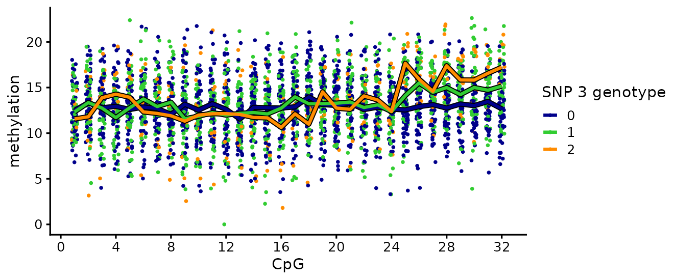
The lines diverge over CpGs 25-32: each additional copy of the SNP 3 alternate allele lifts the methylation level there. At the other CpGs the lines run together; SNP 3 has no direct effect outside its causal cluster.
Per-CpG association tests
A common QTL-mapping recipe runs a separate association test for
every CpG-SNP pair. Below we use the linear regression function
lm(). Plotting the resulting -log10(p-value)
matrix in two views (one per SNP, one per CpG) gives a SNP-centred and a
CpG-centred picture of the signal.
assoc <- matrix(0, T_m, p)
for (i in seq_len(T_m)) {
  for (j in seq_len(p)) {
    assoc[i, j] <- summary(lm(Y[, i] ~ X[, j]))$coefficients[2L, 4L]
  }
}
threshold <- -log10(0.05 / (T_m * p))
pdat_a <- data.frame(
  cpg    = rep(seq_len(T_m), times = p),
  snp    = rep(seq_len(p),   each = T_m),
  effect = as.vector(t(dnam_example$causal_betas[
              match(seq_len(p), dnam_example$causal_snps), ,
              drop = FALSE]) != 0),
  pval   = as.vector(assoc))
pdat_a <- transform(pdat_a, pval = -log10(pval))
pdat_a$effect[is.na(pdat_a$effect)] <- FALSE
p_snp <- ggplot(pdat_a, aes(x = snp, y = pval,
                            shape = effect, color = effect)) +
  geom_point(size = 1.5) +
  geom_hline(yintercept = threshold, color = "black",
             linetype = "dotted") +
  scale_x_continuous(breaks = seq_len(p)) +
  scale_shape_manual(values = c(1, 4)) +
  scale_color_manual(values = c("darkblue", "darkorange")) +
  labs(x = "SNP", y = "-log10 p-value") +
  theme_cowplot(font_size = 10)
p_cpg <- ggplot(pdat_a, aes(x = cpg, y = pval,
                            shape = effect, color = effect)) +
  geom_point(size = 1.5) +
  geom_hline(yintercept = threshold, color = "black",
             linetype = "dotted") +
  scale_x_continuous(breaks = c(0, seq(4, T_m, 4))) +
  scale_shape_manual(values = c(1, 4)) +
  scale_color_manual(values = c("darkblue", "darkorange")) +
  labs(x = "CpG", y = "-log10 p-value") +
  theme_cowplot(font_size = 10)
plot_grid(p_snp, p_cpg, nrow = 1L)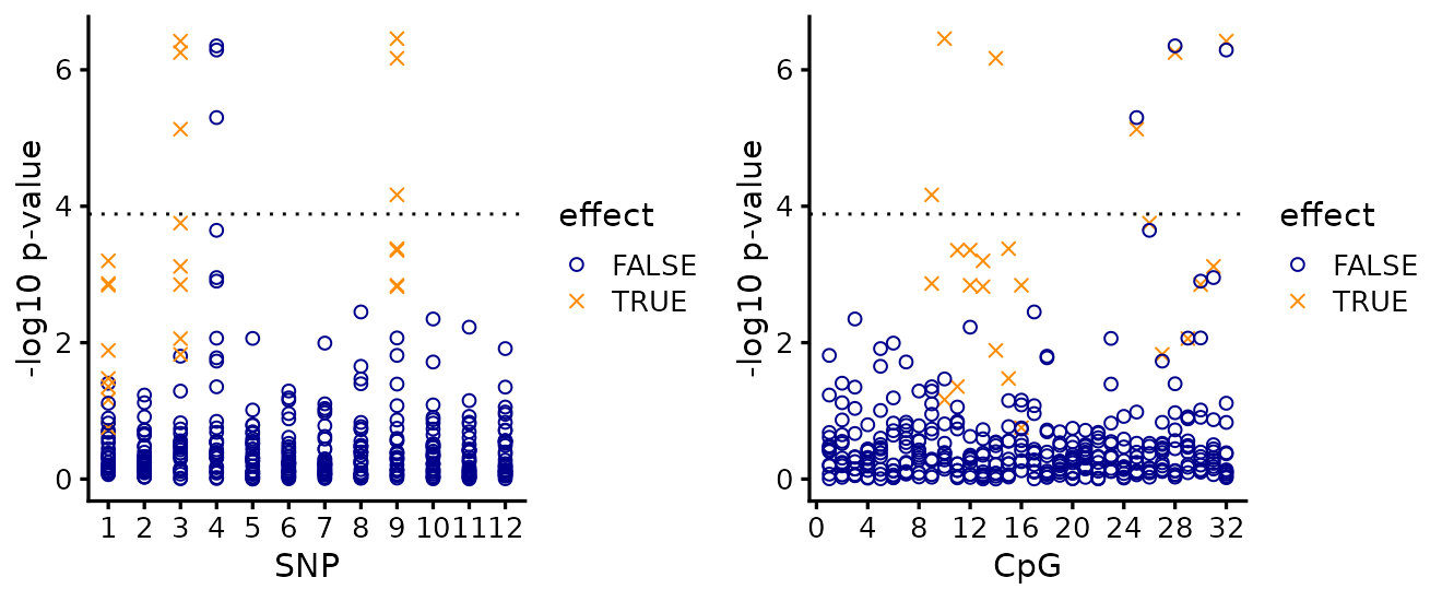
The SNP-centred view (left) hits Bonferroni significance
(-log10(0.05 / (T*p))) at two of the three causal SNPs and
is unable to separate SNP 3 from its high-LD partner SNP 4. But more
importantly, this view alone does not tell us which CpGs are
affected by the SNPs.
The CpG-centred view (right) shows that the affected CpGs cluster in two contiguous regions, but it is less clear which CpG sites in these clusters are actually affected. And this view does not tell us which SNPs drive the changes in methylation at those CpGs.
Per-CpG SuSiE
A natural follow-up is to run SuSiE separately on each associated CpG. This produces one fine-mapping signal per CpG, but leaves the user to integrate them.
assoc_cpgs <- sort(unique(subset(pdat_a, pval > threshold)$cpg))
susie_fits <- lapply(assoc_cpgs, function(i)
  susieR::susie(X, Y[, i], L = 3L))
pdat_s <- do.call(rbind, lapply(seq_along(assoc_cpgs), function(k) {
  data.frame(cpg = assoc_cpgs[k], snp = seq_len(p),
             pip = susie_fits[[k]]$pip)
}))
# Color by cluster membership, with one entry per associated
# CpG. CpGs in cluster A (positions <= 16) are red; cluster B
# (positions > 16) is darkblue. The shape cycles through three
# pchs per cluster so multiple CpGs at the same SNP are
# visually separable.
cpg_levels <- sort(unique(pdat_s$cpg))
pal_levels <- ifelse(cpg_levels < 17L, "red", "darkblue")
shape_cycle <- rep(c(1L, 20L, 4L),
                   length.out = length(cpg_levels))
pdat_s$cpg <- factor(pdat_s$cpg, levels = cpg_levels)
p_susie <- ggplot(pdat_s, aes(x = snp, y = pip,
                              color = cpg, shape = cpg)) +
  geom_point(size = 1.5) +
  scale_color_manual(values = pal_levels) +
  scale_shape_manual(values = shape_cycle) +
  scale_x_continuous(breaks = seq_len(p)) +
  scale_y_continuous(breaks = c(0, 0.5, 1)) +
  labs(x = "SNP", y = "PIP", color = "CpG", shape = "CpG") +
  theme_cowplot(font_size = 10)
print(p_susie)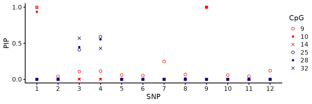
Running susie() on each associated CpG independently
gives one fine-mapping signal per CpG. Two takeaways:
- The signals do not all agree. SNP 1 is identified for the CpGs in cluster A with PIP near 1 (consistent recovery), but for cluster B some CpGs prefer SNP 3 and others SNP 4 — the high-LD partner ambiguity is unresolved in any single fit.
- More importantly, none of the per-CpG SuSiE fits tells us which CpGs are affected by each causal SNP. The output is per-CpG PIPs, not per-SNP affected-CpG sets. fSuSiE solves this directly.
fSuSiE
A single fsusie() call recovers all three causal SNPs in
three credible sets. HMM post-processing produces the per-CpG local
false sign rate (lfsr), which the bubble plot below uses.
fit <- fsusie(Y, X)
fit$sets$cs
#> $L1
#> [1] 9
#>
#> $L3
#> [1] 1
#>
#> $L2
#> [1] 3 4
fit$pip[dnam_example$causal_snps]
#> [1] 1.0000000 1.0000000 0.5632379
fit_h <- mf_post_smooth(fit, method = "HMM")
plot_dims_h <- mfsusie_plot_dimensions(fit_h)
mfsusie_plot(fit_h, effect_variables = dnam_example$causal_snps)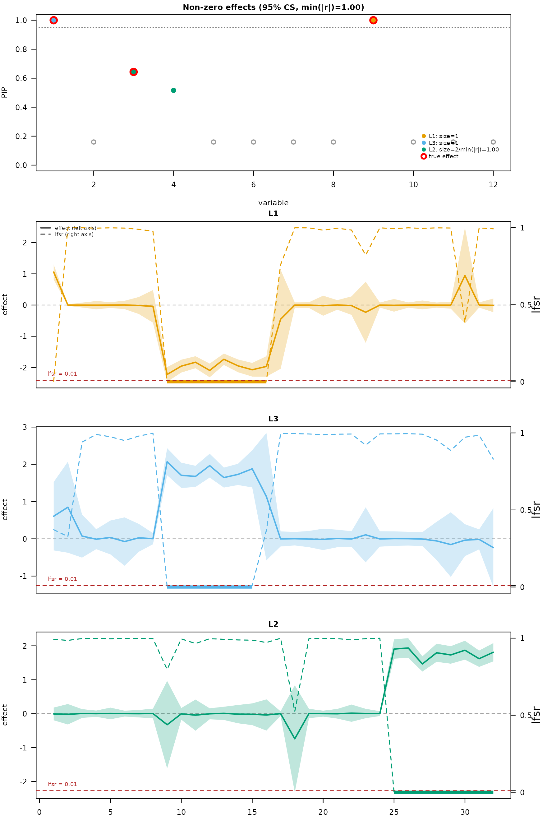
The PIP panel shows three sharp peaks at the causal SNPs. The effect panel rows decompose the per-CS effects across CpGs under HMM post-processing.
Local-false sign rate of effect sizes
mfsusie_plot_lfsr() shows the per-CpG local false sign
rate as a bubble grid. Rows are credible sets, columns are CpGs, dot
size is -log10(lfsr) clamped to [0, cex_max].
Color behavior depends on whether truth is supplied:
- Without
truth: dots at CpGs wherelfsr <= lfsr_threshold(default 0.01) get the CS color; the rest are grey. - With
truth: dots at the truly-affected CpGs get the CS color; the rest are grey, regardless of lfsr.
The simulated truth_mask is indexed by causal SNP (SNPs
1, 3, 9). The fit’s CS order is determined by IBSS and may not match.
The mapping below pulls the right truth mask for each CS by matching its
lead variant to the causal SNPs:
truth_per_cs <- lapply(fit_h$sets$cs, function(cs_vars) {
  hit <- intersect(cs_vars, dnam_example$causal_snps)
  if (length(hit) == 0L) return(rep(FALSE, T_m))
  k <- match(hit[1L], dnam_example$causal_snps)
  dnam_example$truth_mask[[k]]
})
lfsr_dims <- mfsusie_plot_lfsr_dimensions(fit_h)
mfsusie_plot_lfsr(fit_h, truth = truth_per_cs)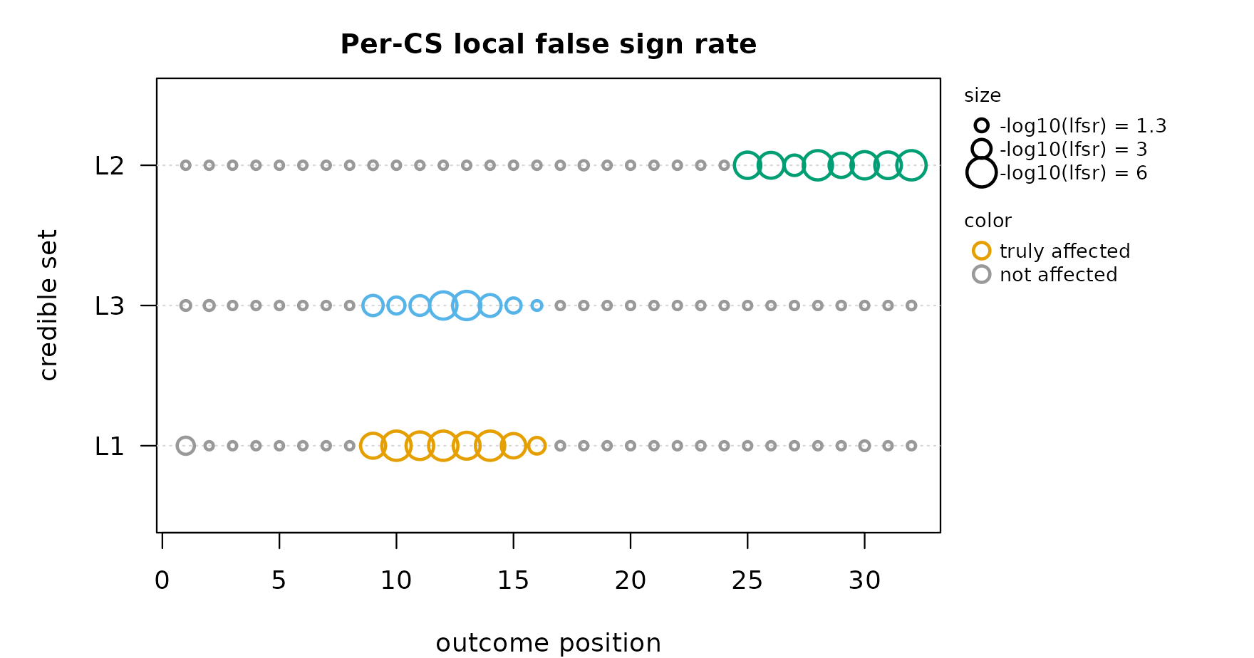
CSes 1 and 2 cover CpGs 9-16; CS 3 covers CpGs 25-32. Both clusters are recovered cleanly. The legend in the upper-right shows the dot-size scale; the lower-right indicates the color rule.
TI-smoothed effects with errorbars
A second post-processing run with the translation-invariant smoother gives pointwise credible bands for each per-CpG effect:
fit_TI <- mf_post_smooth(fit)
range(fit_h$pip - fit_TI$pip)
#> [1] 0 0
plot_dims_ti <- mfsusie_plot_dimensions(fit_TI, facet_cs = "stack")
mfsusie_plot(fit_TI, effect_style = "errorbar", facet_cs = "stack",
             effect_variables = dnam_example$causal_snps)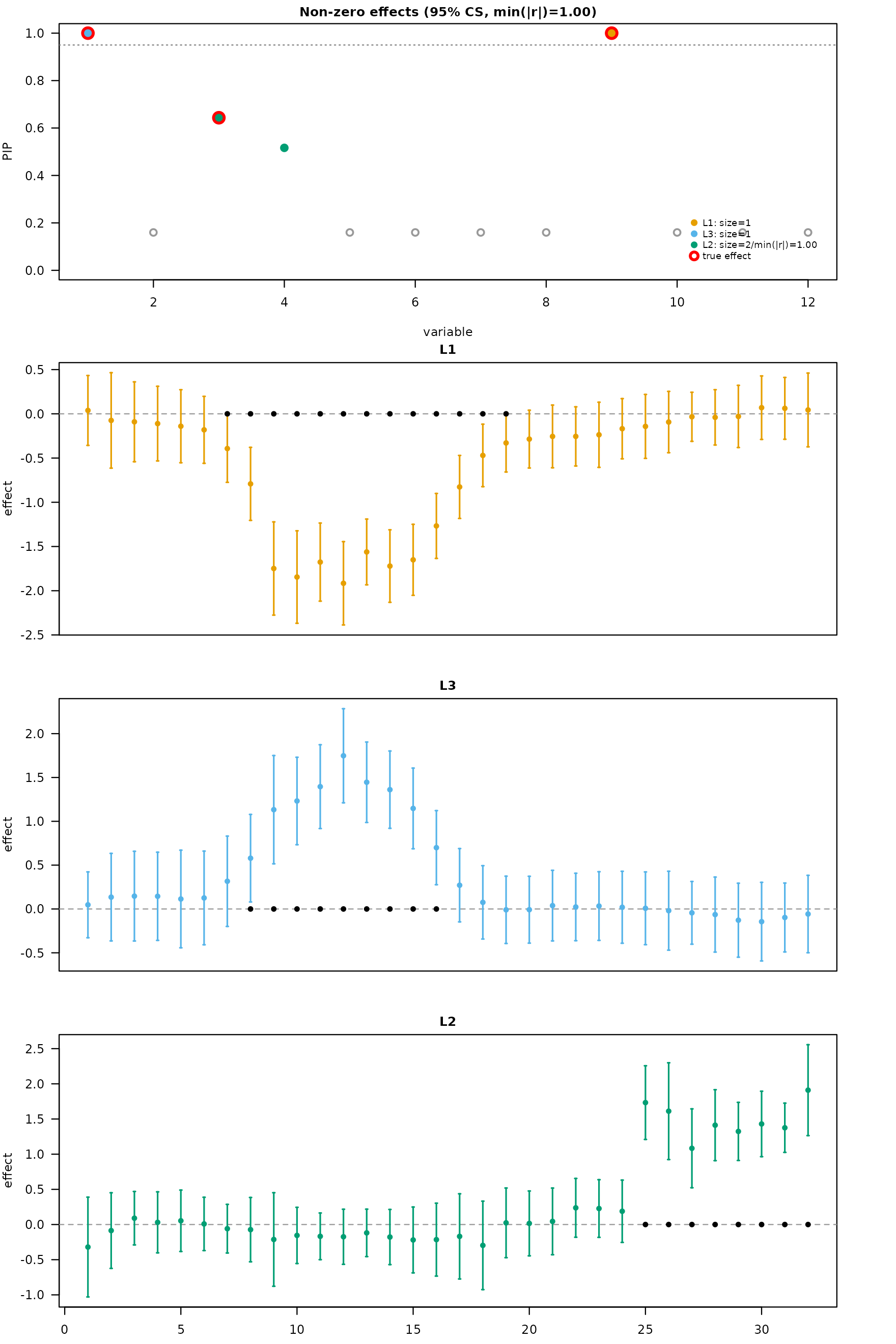
Each row is one CS. The dot at each CpG is the posterior mean effect; the vertical bar is the 95% credible band. Black dots on the zero line mark CpGs where the band excludes zero (the estimated affected CpGs). These align with the ground-truth clusters from the simulation.
Session info
This is the version of R and the packages that were used to generate these results.
sessionInfo()
#> R version 4.4.3 (2025-02-28)
#> Platform: x86_64-conda-linux-gnu
#> Running under: Ubuntu 24.04.4 LTS
#>
#> Matrix products: default
#> BLAS/LAPACK: /home/runner/work/mfsusieR/mfsusieR/.pixi/envs/r44/lib/libopenblasp-r0.3.32.so;  LAPACK version 3.12.0
#>
#> locale:
#>  [1] LC_CTYPE=C.UTF-8       LC_NUMERIC=C           LC_TIME=C.UTF-8
#>  [4] LC_COLLATE=C.UTF-8     LC_MONETARY=C.UTF-8    LC_MESSAGES=C.UTF-8
#>  [7] LC_PAPER=C.UTF-8       LC_NAME=C              LC_ADDRESS=C
#> [10] LC_TELEPHONE=C         LC_MEASUREMENT=C.UTF-8 LC_IDENTIFICATION=C
#>
#> time zone: Etc/UTC
#> tzcode source: system (glibc)
#>
#> attached base packages:
#> [1] stats     graphics  grDevices utils     datasets  methods   base
#>
#> other attached packages:
#> [1] reshape2_1.4.5 cowplot_1.2.0  ggplot2_4.0.3  susieR_0.16.1  mfsusieR_0.0.2
#>
#> loaded via a namespace (and not attached):
#>  [1] gtable_0.3.6          xfun_0.57             bslib_0.10.0
#>  [4] htmlwidgets_1.6.4     ebnm_1.0-55           lattice_0.22-9
#>  [7] vctrs_0.7.3           tools_4.4.3           generics_0.1.4
#> [10] parallel_4.4.3        tibble_3.3.1          pkgconfig_2.0.3
#> [13] Matrix_1.7-5          SQUAREM_2026.1        RColorBrewer_1.1-3
#> [16] S7_0.2.2              desc_1.4.3            RcppParallel_5.1.11-2
#> [19] lifecycle_1.0.5       truncnorm_1.0-9       compiler_4.4.3
#> [22] farver_2.1.2          stringr_1.6.0         textshaping_1.0.5
#> [25] wavethresh_4.7.3      htmltools_0.5.9       sass_0.4.10
#> [28] yaml_2.3.12           pillar_1.11.1         pkgdown_2.2.0
#> [31] crayon_1.5.3          jquerylib_0.1.4       MASS_7.3-65
#> [34] cachem_1.1.0          trust_0.1-9           tidyselect_1.2.1
#> [37] digest_0.6.39         stringi_1.8.7         dplyr_1.2.1
#> [40] LaplacesDemon_16.1.8  ashr_2.2-63           labeling_0.4.3
#> [43] splines_4.4.3         fastmap_1.2.0         grid_4.4.3
#> [46] cli_3.6.6             invgamma_1.2          magrittr_2.0.5
#> [49] dichromat_2.0-0.1     Rfast_2.1.5.2         withr_3.0.2
#> [52] scales_1.4.0          horseshoe_0.2.0       rmarkdown_2.31
#> [55] matrixStats_1.5.0     otel_0.2.0            deconvolveR_1.2-1
#> [58] ragg_1.5.2            evaluate_1.0.5        knitr_1.51
#> [61] irlba_2.3.7           rlang_1.2.0           zigg_0.0.2
#> [64] Rcpp_1.1.1-1.1        mixsqp_0.3-54         glue_1.8.1
#> [67] reshape_0.8.10        jsonlite_2.0.0        R6_2.6.1
#> [70] plyr_1.8.9            systemfonts_1.3.2     fs_2.1.0