Functional fine-mapping with fSuSiE
William Denault
Source:vignettes/fsusie_intro.Rmd
fsusie_intro.RmdOverview
fSuSiE extends the SuSiE Bayesian variable selection model to functional traits. The functional response is sampled at multiple positions of a regular grid (e.g., methylation along a CpG island, RNA-seq coverage along a gene body, ATAC-seq across a peak, ChIP-seq read counts on a window). fSuSiE places a wavelet-basis prior on the per-position effect of each variant and performs sparse variable selection by the SuSiE iterative Bayesian stepwise selection (IBSS) algorithm.
The model is
{\bf Y} = {\bf X} {\bf B} + {\bf E},
where {\bf Y} is n x T
(functional response), {\bf X} is
n x p (genotypes), and {\bf
B} is p x T with most rows zero (few causal
variants). fSuSiE writes {\bf B} as a
sum of single-effect matrices {\bf B} =
\sum_{l=1}^L {\bf B}^{(l)} where each {\bf B}^{(l)} has at most one non-zero row,
then fits the model in the wavelet domain.
fsusie() is the single-outcome wrapper around
mfsusie(). The argument order is
(Y, X, pos, ...).
Example data
library(mfsusieR)
data(coverage_example)
str(coverage_example, max.level = 1)
#> List of 6
#>  $ X           : num [1:574, 1:100] -0.0209 -0.0209 -0.0209 -0.0209 -0.0209 ...
#>  $ Y           : num [1:574, 1:128] 3.024 0.242 -0.658 0.505 -1.734 ...
#>  $ pos         : int [1:128] 1 2 3 4 5 6 7 8 9 10 ...
#>  $ causal_snps : int [1:2] 25 75
#>  $ causal_betas: num [1:2, 1:128] 1.93 -1.36 2.34 -1.31 1.81 ...
#>  $ description : chr "Simulated coverage-QTL example. n = 574, p = 100 SNPs from the susieR::N3finemapping cis window, T = 128 evenly"| __truncated__
coverage_example$causal_snps
#> [1] 25 75
The data are simulated cis-QTL coverage on a power-of-two grid
(n = 574, p = 100, T = 128). The
genotype matrix is the LD scaffold from
susieR::N3finemapping$X[, 1:100]. Two causal SNPs at
positions 25 and 75 carry smooth random per-position effects sampled
from the IBSS wavelet prior, the same prior class fSuSiE assumes. The
setup is assay-agnostic: the per-position response could be RNA-seq
exon-body coverage, ATAC-seq peak coverage, or WGBS / ChIP-seq read
counts on a window.
plot(coverage_example$causal_betas[1L, ], type = "l",
     col = "#1f78b4", lwd = 2,
     ylim = range(coverage_example$causal_betas),
     xlab = "position", ylab = "effect")
abline(h = 0, lty = 3, col = "grey50")
lines(coverage_example$causal_betas[2L, ], col = "#33a02c", lwd = 2)
legend("topright",
       legend = paste0("variable ", coverage_example$causal_snps),
       col = c("#1f78b4", "#33a02c"), lwd = 2, bty = "n")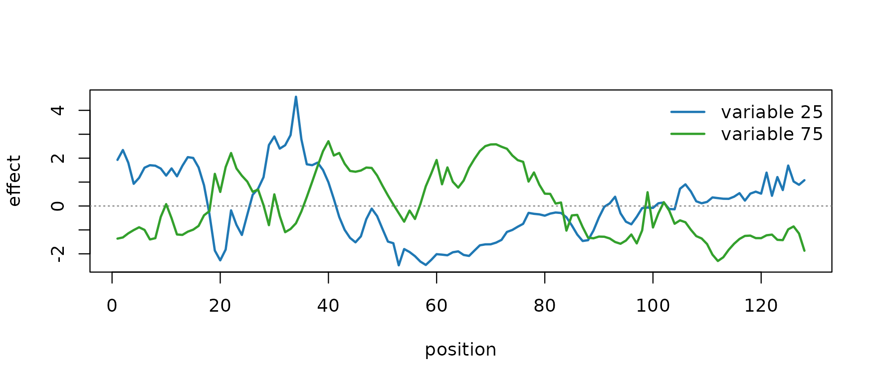
Fitting fSuSiE
fit <- fsusie(coverage_example$Y, coverage_example$X,
              pos = coverage_example$pos)
fit$niter; fit$converged
#> [1] 2
#> [1] TRUE
fit$sets$cs
#> $L1
#> [1] 75 83
#>
#> $L2
#> [1] 25
fit$pip[coverage_example$causal_snps]
#> [1] 1.0 0.5
Both causal SNPs receive PIP near 1 and land in two separate credible sets.
Visualizing the fit
mfsusie_plot() returns a two-panel layout for
single-outcome fits: PIPs on top, per-CS effect curves on the bottom.
With facet_cs = "auto" (the default) two CSes whose
affected regions are disjoint are stacked into separate rows.
plot_dims_raw <- mfsusie_plot_dimensions(fit)
plot_dims_raw
#> $width
#> [1] 8
#>
#> $height
#> [1] 6
#>
#> $n_cells
#> [1] 2
mfsusie_plot(fit, effect_variables = coverage_example$causal_snps)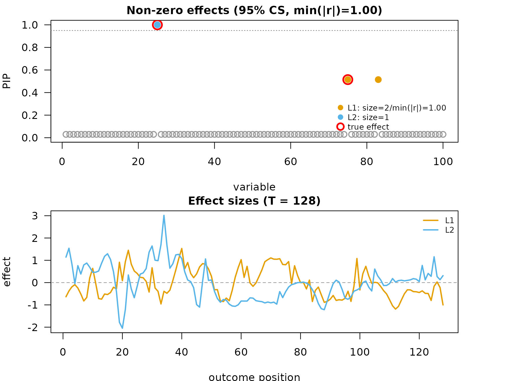
The raw inverse-DWT effect curves track the true shapes but carry
high-frequency content from the finest wavelet scales. The default
"TI" smoother (cycle-spinning translation- invariant
wavelet denoising) trims that content and adds a pointwise 95% credible
band.
fit_s <- mf_post_smooth(fit)
plot_dims_s <- mfsusie_plot_dimensions(fit_s)
plot_dims_s
#> $width
#> [1] 8
#>
#> $height
#> [1] 6
#>
#> $n_cells
#> [1] 2
mfsusie_plot(fit_s, effect_variables = coverage_example$causal_snps)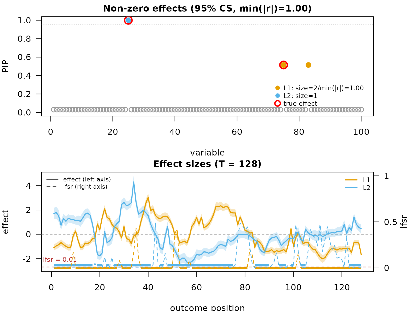
mf_post_smooth() exposes other smoothers
("scalewise", "HMM", "smash") and
their tunable parameters; see vignette("post_processing")
for the comparison.
The errorbar style draws a per-position dot at the posterior mean and a vertical bar to the credible band.
plot_dims_eb <- mfsusie_plot_dimensions(fit_s, facet_cs = "stack")
mfsusie_plot(fit_s, effect_style = "errorbar", facet_cs = "stack",
             effect_variables = coverage_example$causal_snps)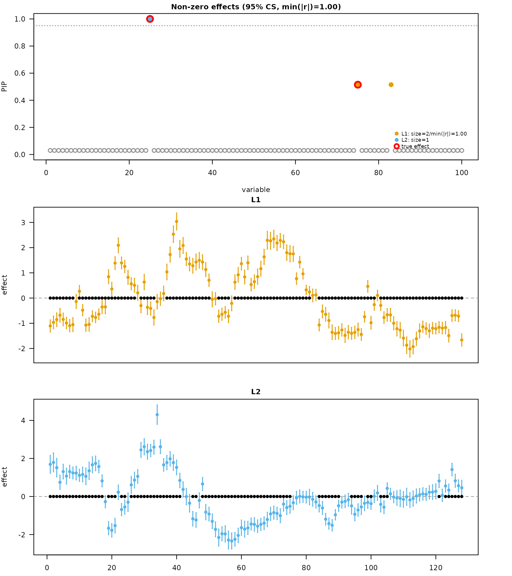
Recovering the true effect
Overlay the TI-smoothed effect against the truth to verify recovery on each causal SNP. The truth is a per-position discrete value, so render it as dots rather than a curve.
truth <- coverage_example$causal_betas
band  <- fit_s$smoothed$TI$credible_bands

# Match each fitted CS to its causal SNP by lead PIP.
cs_lead <- vapply(fit$sets$cs, function(idx) {
  idx[which.max(fit$pip[idx])]
}, integer(1L))

par(mfrow = c(1L, length(cs_lead)),
    mar = c(4, 4, 2.5, 1))
for (i in seq_along(cs_lead)) {
  truth_idx <- match(cs_lead[i], coverage_example$causal_snps)
  pos_grid  <- coverage_example$pos
  b_i       <- band[[1L]][[i]]
  rec_i     <- fit_s$smoothed$TI$effect_curves[[1L]][[i]]
  yrng      <- range(b_i, truth[truth_idx, ], rec_i, na.rm = TRUE)
  plot(pos_grid, truth[truth_idx, ], pch = 20L, col = "grey30",
       cex = 0.7,
       xlab = "position", ylab = "effect",
       ylim = yrng,
       main = sprintf("CS %d (SNP %d)", i, cs_lead[i]))
  polygon(c(pos_grid, rev(pos_grid)),
          c(b_i[, 1L], rev(b_i[, 2L])),
          col = adjustcolor("#1f78b4", alpha.f = 0.25),
          border = NA)
  lines(pos_grid, rec_i, col = "#1f78b4", lwd = 2)
  abline(h = 0, lty = 3, col = "grey50")
  legend("topright", legend = c("truth", "TI smooth", "95% band"),
         col    = c("grey30", "#1f78b4", adjustcolor("#1f78b4", alpha.f = 0.5)),
         lty    = c(NA, 1, NA), lwd = c(NA, 2, NA),
         pch    = c(20, NA, 15), bty = "n", cex = 0.75)
}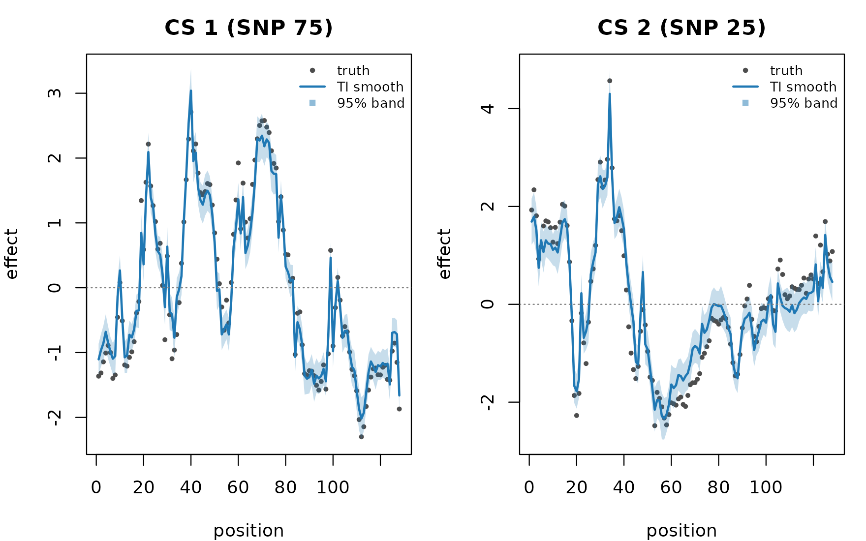
The TI-smoothed curve tracks the truth across the support; the 95% band covers the per-position truth at most sites and only crosses the band on the small high-frequency wiggles the smoother trims.
Uneven sampling positions
Wavelets assume a 2^J evenly-spaced grid.
fsusie() accepts unevenly-spaced positions by remapping the
data onto a regular dyadic grid with the Kovac-Silverman procedure. Pass
the positions through the pos argument; the response is
interpolated internally and the fit returns the per-position effect on
the remapped grid.
To illustrate, drop a random subset of positions from the evenly-spaced response and refit on the irregular grid:
set.seed(2)
T_full   <- ncol(coverage_example$Y)
keep     <- sort(sample.int(T_full, size = 100L, replace = FALSE))
Y_uneven <- coverage_example$Y[, keep]
fit_uneven <- fsusie(Y_uneven, coverage_example$X,
                     pos = keep)
fit_uneven$sets$cs
#> $L1
#> [1] 75 83
#>
#> $L2
#> [1] 25
fit_uneven$pip[coverage_example$causal_snps]
#> [1] 1.0 0.5
fit_uneven_s <- mf_post_smooth(fit_uneven)
plot_dims_u <- mfsusie_plot_dimensions(fit_uneven_s)
mfsusie_plot(fit_uneven_s, effect_variables = coverage_example$causal_snps)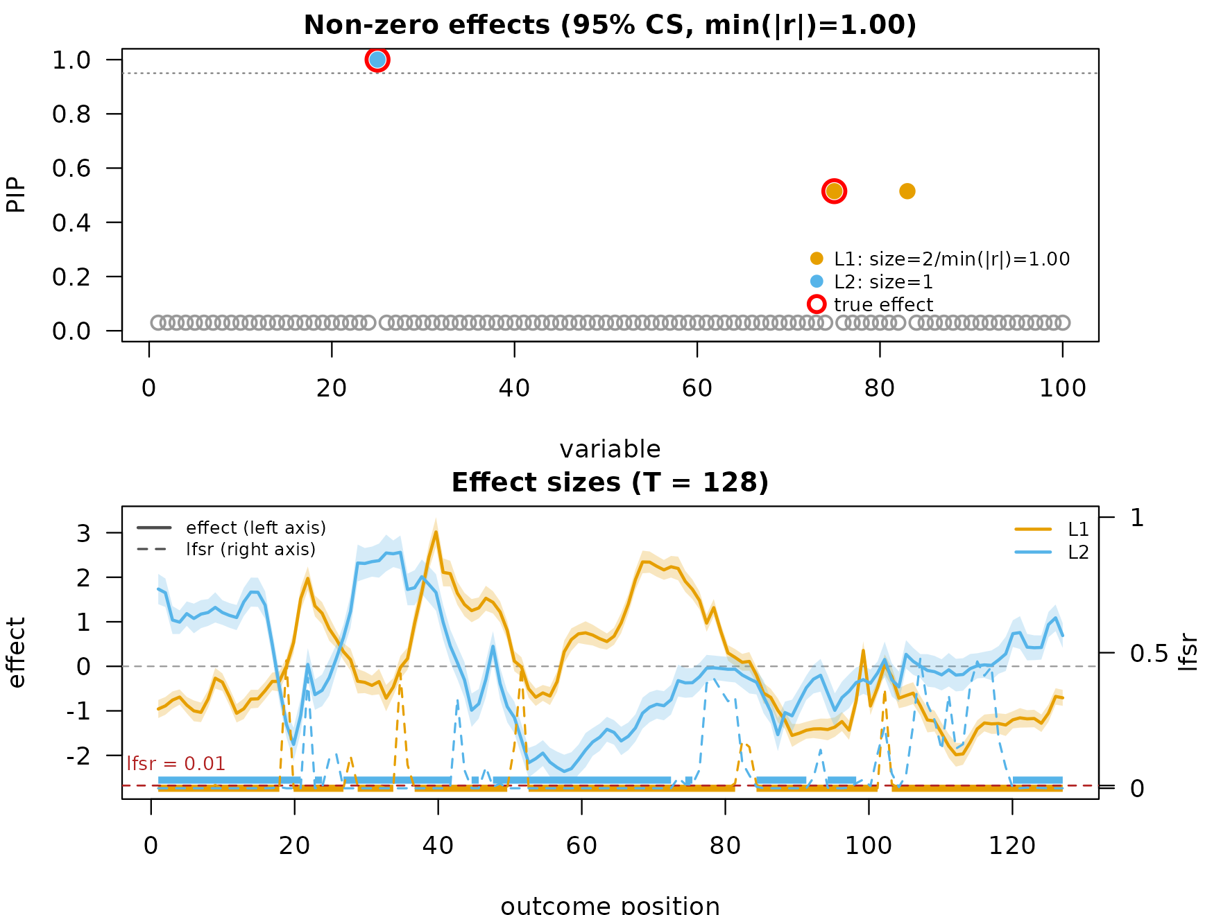
The credible bands are wider than in the evenly-sampled fit because each position now contributes information at a non-uniform local density.
Prior choices
The wavelet-domain mixture prior on {\bf B}^{(l)} has three options that trade flexibility, sample-size efficiency, and runtime:
-
prior_variance_scope = "per_outcome"(default): one K+1-component scale-mixture-of-normals per outcome, with weights pooled across all wavelet scales. Fit bymixsqp. Cheapest per IBSS iteration. -
prior_variance_scope = "per_scale": a separate K+1-component mixture per (outcome, scale). Fit bymixsqp. Helps when the signal magnitude varies systematically with scale, at roughlyS_m-fold moremixsqpcalls per IBSS iteration. -
prior_variance_scope = "per_scale_normal": a 2-component point-Normal spike-and-slab per (outcome, scale), fit byebnm::ebnm_point_normal(). Two parameters per (outcome, scale) cell:pi_0(null mass) andsigma(slab standard deviation).
The rationale for per_scale_normal: within a single
wavelet scale s the coefficients share a characteristic
effect-size scale, so a 2-parameter spike-and-slab is the right Bayesian
model. With two parameters per cell instead of the K+1 ≈ 30 of
per_scale, the data goes ~15x further per fitted parameter,
and the parametric form is intrinsically regularized (no
mixture_null_weight knob is consumed). A companion option
prior_variance_scope = "per_scale_laplace" swaps the Normal
slab for a Laplace slab and accommodates sparse-within-scale signals
(1-2 active positions out of the scale’s grid).
Fit all three on the example:
fit_per_out   <- fsusie(coverage_example$Y, coverage_example$X,
                        pos = coverage_example$pos)             # per_outcome (default)
fit_per_scale <- fsusie(coverage_example$Y, coverage_example$X,
                        pos = coverage_example$pos,
                        prior_variance_scope = "per_scale")
fit_per_scale_n <- fsusie(coverage_example$Y, coverage_example$X,
                          pos = coverage_example$pos,
                          prior_variance_scope = "per_scale_normal")
c(per_outcome      = fit_per_out$niter,
  per_scale        = fit_per_scale$niter,
  per_scale_normal = fit_per_scale_n$niter)
#>      per_outcome        per_scale per_scale_normal
#>                2                5                4
Pairwise PIP comparison in two panels: per_scale vs
per_outcome (left), per_scale_normal vs
per_scale (right).
par(mfrow = c(1L, 2L), mar = c(4, 4, 2.5, 1))
plot(fit_per_out$pip, fit_per_scale$pip,
     pch = 16, cex = 0.8, col = "#1f78b4",
     xlab = "PIP (per_outcome, default)",
     ylab = "PIP (per_scale)",
     xlim = c(0, 1), ylim = c(0, 1),
     main = "per_scale vs per_outcome")
abline(0, 1, lty = 3, col = "grey50")
plot(fit_per_scale$pip, fit_per_scale_n$pip,
     pch = 16, cex = 0.8, col = "#1f78b4",
     xlab = "PIP (per_scale)",
     ylab = "PIP (per_scale_normal)",
     xlim = c(0, 1), ylim = c(0, 1),
     main = "per_scale_normal vs per_scale")
abline(0, 1, lty = 3, col = "grey50")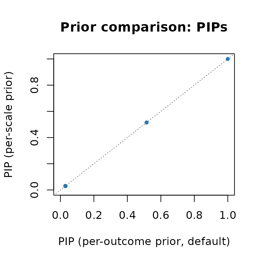
The three priors put the causal mass on the same variants; PIPs sit
on the diagonal for the lead variants in each credible set. Pick
per_outcome for the cheapest fit, per_scale
when scale-heterogeneous shape is important, and
per_scale_normal when each wavelet scale has a single
characteristic effect-size scale and the K+1-component
mixsqp fit is under-determined on coarse scales.
Wavelet-domain preprocessing
fsusie() exposes three preprocessing flags for the
wavelet matrix:
-
wavelet_magnitude_cutoff(default0): wavelet columns withmedian(|column|) <= wavelet_magnitude_cutoffare masked, contributing(Bhat = 0, Shat = 1)to the SER step. Use a small positive value when the response has sparse non-zero entries (e.g., ATAC-seq read pileups). -
wavelet_standardize(defaultTRUE): centers and scales each packed wavelet coefficient column before IBSS, then maps fitted values and coefficients back through that linear scaling. -
wavelet_qnorm(defaultFALSE): applies a column-wise rank-based normal quantile transform to the wavelet matrix. Useful when the per-position residuals are heavy-tailed or visibly non-Gaussian. Leave itFALSEto skip the transform when the wavelet coefficients are already approximately Gaussian.
See ?mfsusie for the full set of preprocessing
options.
What the fit object carries
str(fit, max.level = 1)
#> List of 32
#>  $ alpha                 : num [1:5, 1:100] 0 0 0.01 0.01 0.01 0 0 0.01 0.01 0.01 ...
#>  $ mu                    :List of 5
#>  $ mu2                   :List of 5
#>  $ V                     : num [1:5] 0.0314 0.0211 0 0 0
#>  $ V_grid                :List of 1
#>  $ pi_V                  :List of 5
#>  $ null_prior_init       : num 0
#>  $ G_prior               :List of 1
#>  $ fitted_g_per_effect   :List of 5
#>  $ cross_outcome_combiner: list()
#>   ..- attr(*, "class")= chr [1:2] "mf_prior_cross_outcome_independent" "mf_prior_cross_outcome"
#>  $ KL                    : num [1:5] 139 107 0 0 0
#>  $ lbf                   : num [1:5] 1046 791 0 0 0
#>  $ lbf_variable          : num [1:5, 1:100] -23.3 -22.2 0 0 0 ...
#>  $ lbf_variable_outcome  : num [1:5, 1:100, 1] -23.3 -22.2 0 0 0 ...
#>  $ sigma2                :List of 1
#>  $ pi                    : num [1:100] 0.01 0.01 0.01 0.01 0.01 0.01 0.01 0.01 0.01 0.01 ...
#>  $ fitted                :List of 1
#>  $ intercept             :List of 1
#>  $ L                     : int 5
#>  $ p                     : int 100
#>  $ M                     : int 1
#>  $ null_index            : num 0
#>  $ converged             : logi TRUE
#>  $ convergence_reason    : chr "alpha_pip_fixed_point"
#>  $ elbo                  : num [1:2] NA -102473
#>  $ niter                 : int 2
#>  $ X_column_scale_factors: num [1:100] 0.143 0.624 0.684 0.23 0.411 ...
#>  $ sets                  :List of 5
#>  $ pip                   : num [1:100] 0 0 0 0 0 0 0 0 0 0 ...
#>  $ Y_grid                :List of 1
#>  $ X_eff                 :List of 5
#>  $ dwt_meta              :List of 14
#>  - attr(*, "class")= chr [1:2] "mfsusie" "susie"
The fit is a list of class c("mfsusie", "susie") with
the standard SuSiE slots (alpha, mu,
mu2, lbf, lbf_variable,
KL, pip, sets) plus per-outcome
wavelet metadata (dwt_meta) used by
predict.mfsusie, coef.mfsusie, and
fitted.mfsusie. After
mf_post_smooth(fit, method = ...), the chosen smoother’s
output lives at fit$smoothed[[method]] (with
effect_curves, credible_bands, and an optional
lfsr_curves slot for HMM). The fit accumulates per-method
results across calls, so multiple smoothers can coexist on the same fit;
see vignette("post_processing") for the comparison
workflow. mfsusie_plot() picks a smoother by priority
TI > smash > HMM > scalewise when more than one is
present.
Session info
This is the version of R and the packages that were used to generate these results.
sessionInfo()
#> R version 4.4.3 (2025-02-28)
#> Platform: x86_64-conda-linux-gnu
#> Running under: Ubuntu 24.04.4 LTS
#>
#> Matrix products: default
#> BLAS/LAPACK: /home/runner/work/mfsusieR/mfsusieR/.pixi/envs/r44/lib/libopenblasp-r0.3.32.so;  LAPACK version 3.12.0
#>
#> locale:
#>  [1] LC_CTYPE=C.UTF-8       LC_NUMERIC=C           LC_TIME=C.UTF-8
#>  [4] LC_COLLATE=C.UTF-8     LC_MONETARY=C.UTF-8    LC_MESSAGES=C.UTF-8
#>  [7] LC_PAPER=C.UTF-8       LC_NAME=C              LC_ADDRESS=C
#> [10] LC_TELEPHONE=C         LC_MEASUREMENT=C.UTF-8 LC_IDENTIFICATION=C
#>
#> time zone: Etc/UTC
#> tzcode source: system (glibc)
#>
#> attached base packages:
#> [1] stats     graphics  grDevices utils     datasets  methods   base
#>
#> other attached packages:
#> [1] mfsusieR_0.0.2
#>
#> loaded via a namespace (and not attached):
#>  [1] sass_0.4.10           generics_0.1.4        ashr_2.2-63
#>  [4] lattice_0.22-9        digest_0.6.39         magrittr_2.0.5
#>  [7] evaluate_1.0.5        grid_4.4.3            RColorBrewer_1.1-3
#> [10] fastmap_1.2.0         plyr_1.8.9            jsonlite_2.0.0
#> [13] Matrix_1.7-5          reshape_0.8.10        mixsqp_0.3-54
#> [16] scales_1.4.0          truncnorm_1.0-9       invgamma_1.2
#> [19] textshaping_1.0.5     jquerylib_0.1.4       cli_3.6.6
#> [22] crayon_1.5.3          zigg_0.0.2            rlang_1.2.0
#> [25] deconvolveR_1.2-1     susieR_0.16.1         LaplacesDemon_16.1.8
#> [28] splines_4.4.3         cachem_1.1.0          yaml_2.3.12
#> [31] otel_0.2.0            ebnm_1.0-55           tools_4.4.3
#> [34] SQUAREM_2026.1        parallel_4.4.3        dplyr_1.2.1
#> [37] wavethresh_4.7.3      ggplot2_4.0.3         Rfast_2.1.5.2
#> [40] vctrs_0.7.3           R6_2.6.1              matrixStats_1.5.0
#> [43] lifecycle_1.0.5       fs_2.1.0              htmlwidgets_1.6.4
#> [46] MASS_7.3-65           trust_0.1-9           ragg_1.5.2
#> [49] irlba_2.3.7           pkgconfig_2.0.3       desc_1.4.3
#> [52] RcppParallel_5.1.11-2 pkgdown_2.2.0         bslib_0.10.0
#> [55] pillar_1.11.1         gtable_0.3.6          glue_1.8.1
#> [58] Rcpp_1.1.1-1.1        systemfonts_1.3.2     xfun_0.57
#> [61] tibble_3.3.1          tidyselect_1.2.1      dichromat_2.0-0.1
#> [64] knitr_1.51            farver_2.1.2          htmltools_0.5.9
#> [67] rmarkdown_2.31        compiler_4.4.3        S7_0.2.2
#> [70] horseshoe_0.2.0