This notebook gives the R functions that runs on a small example.
Download the R notebook (.ipynb). Open it in JupyterLab with an R kernel and run the cells in order.
set.seed(5)
toy_p <- rbind(rep(0.20, 80), rep(0.80, 80))
toy_group <- rep(c('A', 'B'), each = 12)
toy_x <- matrix(0L, nrow = 24, ncol = 80)
for (i in seq_len(nrow(toy_x))) {
  toy_x[i, ] <- rbinom(80, 2, toy_p[match(toy_group[i], c('A', 'B')), ])
}
stopifnot(all(toy_x %in% 0:2))
Main functions
prepare_pca() centers each SNP count and divides by the Hardy–Weinberg standard deviation . fit_ancestry() fits the allele-draw likelihood by an EM algorithm. Read the code before applying it to new data. In particular, check which quantities the functions estimate from the sample.
prepare_pca <- function(genotype, components = 4L) {
  allele_frequency <- colMeans(genotype) / 2
  marker_sd <- sqrt(2 * allele_frequency * (1 - allele_frequency))
  ## Exclude nearly monomorphic SNPs with an unstable scaling denominator.
  keep <- marker_sd > 0.05
  centered <- sweep(genotype[, keep, drop = FALSE], 2,
                    2 * allele_frequency[keep], "-")
  standardized <- sweep(centered, 2, marker_sd[keep], "/")
  fit <- prcomp(standardized, center = FALSE, scale. = FALSE,
                rank. = components)
  variance_fraction <- fit$sdev^2 / sum(fit$sdev^2)
  list(scores = fit$x, allele_frequency = allele_frequency, keep = keep,
       variance_fraction = variance_fraction[seq_len(ncol(fit$x))])
}

fit_ancestry <- function(genotype, k, scores, max_iter = 2000L,
                         per_cell_tol = 1e-7, q_tol = 1e-4) {
  n <- nrow(genotype)
  m <- ncol(genotype)
  centers <- kmeans(scores[, seq_len(min(ncol(scores), 4L)), drop = FALSE],
                    centers = k, nstart = 10L)$cluster
  q <- matrix(0.1 / k, nrow = n, ncol = k)
  q[cbind(seq_len(n), centers)] <- 0.9 + 0.1 / k
  p <- vapply(seq_len(k), function(j) {
    colSums(sweep(genotype, 1, q[, j], "*")) / (2 * sum(q[, j]))
  }, numeric(m))
  p[p < 0.005] <- 0.005
  p[p > 0.995] <- 0.995

  log_likelihood <- numeric(max_iter)
  stable_updates <- 0L
  for (iteration in seq_len(max_iter)) {
    previous_q <- q
    f <- q %*% t(p)
    f[f < 0.001] <- 0.001
    f[f > 0.999] <- 0.999
    copy_count <- matrix(0, n, k)
    allele_count <- matrix(0, m, k)
    source_count <- matrix(0, m, k)

    for (j in seq_len(k)) {
      alt <- sweep(matrix(p[, j], n, m, byrow = TRUE), 1, q[, j], "*") / f
      ref <- sweep(matrix(1 - p[, j], n, m, byrow = TRUE), 1,
                   q[, j], "*") / (1 - f)
      assigned_alt <- genotype * alt
      assigned_ref <- (2 - genotype) * ref
      assigned <- assigned_alt + assigned_ref
      copy_count[, j] <- rowSums(assigned)
      allele_count[, j] <- colSums(assigned_alt)
      source_count[, j] <- colSums(assigned)
    }
    ## Keep a nearly unused source from disappearing numerically.
    q <- pmax(copy_count / (2 * m), 1e-6)
    q <- q / rowSums(q)
    p <- allele_count / source_count
    p[p < 0.005] <- 0.005
    p[p > 0.995] <- 0.995
    ## Record the likelihood after the update, using the returned P and Q.
    log_likelihood[iteration] <- sum(dbinom(genotype, 2, q %*% t(p), log = TRUE))
    if (iteration > 1L) {
      gain <- log_likelihood[iteration] - log_likelihood[iteration - 1L]
      small_change <- abs(gain) / (n * m) < per_cell_tol &&
                      max(abs(q - previous_q)) < q_tol
      stable_updates <- if (small_change) stable_updates + 1L else 0L
      if (stable_updates >= 10L) break
    }
  }
  stopifnot(max(abs(rowSums(q) - 1)) < 1e-8,
            all(p >= 0), all(p <= 1))
  converged <- stable_updates >= 10L
  if (!converged) warning("Iteration limit reached; inspect the trace or increase max_iter.")
  list(q = q, p = p, log_likelihood = log_likelihood[seq_len(iteration)],
       converged = converged, iterations = iteration)
}
toy_pc <- prepare_pca(toy_x)
set.seed(5)
toy_fit <- fit_ancestry(toy_x, k = 2, scores = toy_pc$scores)
par(mfrow = c(1, 2), mar = c(4, 4, 2, 1))
plot(toy_pc$scores[, 1:2], col = as.integer(factor(toy_group)),
     pch = 19, xlab = 'PC1', ylab = 'PC2', main = 'PCA')
barplot(t(toy_fit$q), col = c('#277DA1', '#C03A2B'), border = NA,
        space = 0, axes = FALSE, main = 'Ancestry model, K = 2')
par(mfrow = c(1, 1))
stopifnot(all(diff(toy_fit$log_likelihood) > -1e-6))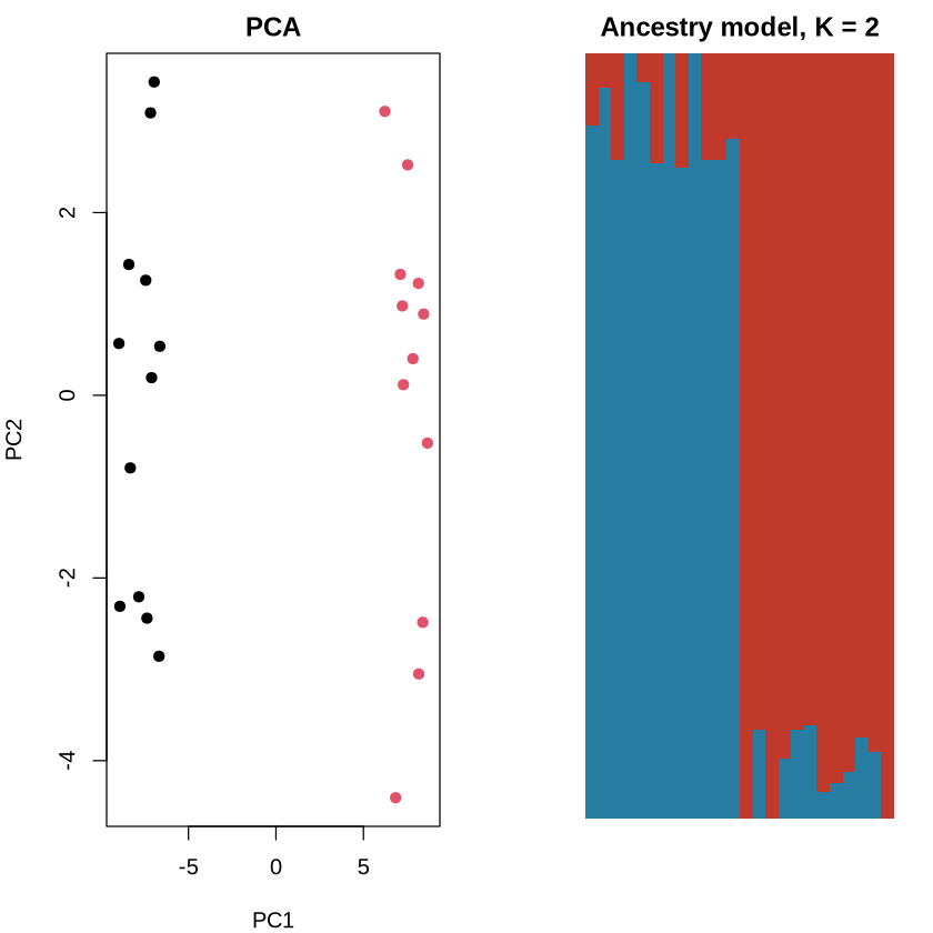
Credits
The five-population teaching question follows Hellenthal, Handbook of Statistical Genomics (2019), Figures 8.2–8.3, which adapt the simulation in Lawson et al. (2012). The homework genotype matrix is a new course simulation, not the published matrix. For the allele-draw model, see Pritchard, An Owner’s Guide to the Human Genome, Chapter 3.1.
- Lawson, D. J., Hellenthal, G., Myers, S., & Falush, D. (2012). Inference of Population Structure using Dense Haplotype Data. PLoS Genetics, 8(1), e1002453. 10.1371/journal.pgen.1002453