Genome-wide kinship - P8149 Computational Vignettes

How do PLINK and KING turn genome-wide identity by state (IBS) into identity by descent (IBD), and when do they agree?

Start from first principles¶

The kinship coefficient $\phi_{ij}$ is the probability that one random allele from person $i$ and one random allele from person $j$ are IBD.

Local IBD asks where a shared segment lies. Genome-wide kinship asks for its average over the genome. At one marker, an IBS match may be accidental. Across many markers, accidental matches approach a predictable baseline; relatives remain more similar because they inherited some of the same ancestral DNA.

1. Why averaging works¶

Start with one haploid copy from each person and 12 independent markers. Let the allele frequency be $p=1/2$ at every marker. Two unrelated copies match by chance with probability

c=p^2+(1-p)^2=\frac12.

(1)

Suppose a fraction $q$ of the two copies is IBD. The alleles must match there. They match with probability $c$ elsewhere. Therefore

P(\mathrm{IBS})=q+(1-q)c, \qquad q=\frac{P(\mathrm{IBS})-c}{1-c}.

(2)

The IBD states below are shown only to check the example. Real genotype data contain the match pattern, not the hidden ancestry state.

marker <- seq_len(12)

unrelated_match <- c(1, 0, 1, 0, 0, 1, 1, 0, 1, 0, 0, 1)
related_ibd_truth <- c(1, 1, 1, 1, rep(0, 8))
related_match <- c(1, 1, 1, 1, 1, 0, 1, 0, 1, 0, 1, 0)

toy_data <- data.frame(
  marker,
  unrelated_IBS_match = unrelated_match,
  related_IBS_match = related_match,
  related_IBD_truth_for_checking = related_ibd_truth
)
toy_data

chance_match <- 0.5
match_rate <- c(mean(unrelated_match), mean(related_match))
estimated_ibd_fraction <- (match_rate - chance_match) / (1 - chance_match)

toy_summary <- data.frame(
  pair = c("Unrelated", "Related"),
  matches = c(sum(unrelated_match), sum(related_match)),
  markers = length(marker),
  match_rate,
  estimated_IBD_fraction = estimated_ibd_fraction
)
toy_summary

stopifnot(estimated_ibd_fraction[1] == 0)
stopifnot(abs(estimated_ibd_fraction[2] - mean(related_ibd_truth)) < 1e-12)

2. PLINK: estimate the IBD mixture¶

For a pair of diploid people, let $K_m\in\{0,1,2\}$ be the number of copies shared IBD at marker $m$ . Across the genome,

K_m\sim\operatorname{Categorical}(Z_0,Z_1,Z_2).

(3)

We do not observe $K_m$ . We observe the IBS count $I_m\in\{0,1,2\}$ . Under HWE with allele frequency $p$ and $r=1-p$ ,

P(I_m\mid K_m,p)= \begin{array}{c|ccc} & K=0 & K=1 & K=2\\ \hline I=0 & 2p^2r^2 & 0 & 0\\ I=1 & 4pr(p^2+r^2) & 2pr & 0\\ I=2 & p^4+r^4+4p^2r^2 & p^2+r^2 & 1 \end{array}.

(4)

PLINK matches the expected and observed IBS 0/1/2 counts across markers to estimate $Z_0,Z_1,Z_2$ . It then reports

\widehat\phi_{ij}^{\mathrm{PLINK}}=\frac14\widehat Z_1+\frac12\widehat Z_2, \qquad \widehat{\mathrm{PI\_HAT}}=2\widehat\phi_{ij}^{\mathrm{PLINK}}.

(5)

The code below implements this basic moment calculation with known allele frequencies. PLINK adds practical safeguards and finite-sample corrections.

3. KING: estimate kinship directly¶

Let $G_{im}\in\{0,1,2\}$ be the allele count and $H_{im}=1(G_{im}=1)$ indicate a heterozygous genotype. KING-robust uses

\widehat\phi_{ij}^{\mathrm{KING}} =\frac12- \frac{\sum_m(G_{im}-G_{jm})^2} {2\sum_m(H_{im}+H_{jm})}.

(6)

The numerator measures how different the two genotypes are. The denominator measures how much variation is available within this pair. It does not depend on who else happens to be in the sample.

4. Their connection¶

A simple frequency-based moment makes the connection visible:

\widehat\phi_{ij}^{\mathrm{frequency}} =\frac12- \frac{\sum_m(G_{im}-G_{jm})^2} {8\sum_m p_m(1-p_m)}.

(7)

This one equation does not recover all three PLINK IBD proportions. But it is exactly the kinship component of the basic PLINK moment calculation: squared genotype difference gives weight 4 to IBS 0, weight 1 to IBS 1, and weight 0 to IBS 2.

E(H_{im}+H_{jm}\mid p_m)=4p_m(1-p_m),

(8)

KING replaces the frequency denominator with pair heterozygosity. Under one homogeneous HWE population, KING’s denominator approaches the frequency denominator as the number of independent markers grows. PLINK and KING then estimate the same target,

\phi_{ij}=\frac14Z_1+\frac12Z_2.

(9)

Thus the basic PLINK and frequency-moment kinship estimates are algebraically the same. KING is different in a finite sample, but has the same large-marker limit when the pooled allele frequencies describe both people.

5. Unrelated pairs and siblings¶

The simulation uses independent SNPs. Unrelated genotypes are sampled independently. Siblings inherit one allele from each of the same two parents. Linkage is omitted because the target is a genome-wide average.

set.seed(8149)

n_markers <- 5000
n_pairs <- 100
allele_frequency <- runif(n_markers, 0.10, 0.50)

plink_ibs_matrix <- function(p) {
  r <- 1 - p
  rbind(
    IBS0 = c(mean(2 * p^2 * r^2), 0, 0),
    IBS1 = c(mean(4 * p * r * (p^2 + r^2)), mean(2 * p * r), 0),
    IBS2 = c(mean(p^4 + r^4 + 4 * p^2 * r^2), mean(p^2 + r^2), 1)
  )
}

estimate_plink <- function(genotype_i, genotype_j, frequency) {
  ibs <- ifelse(genotype_i == genotype_j, 2L,
    ifelse(abs(genotype_i - genotype_j) == 2L, 0L, 1L))
  observed <- tabulate(ibs + 1L, nbins = 3L) / length(ibs)
  z <- drop(solve(plink_ibs_matrix(frequency), observed))
  names(z) <- c("Z0", "Z1", "Z2")
  c(z, kinship = unname(z["Z1"] / 4 + z["Z2"] / 2))
}

estimate_frequency_moment <- function(genotype_i, genotype_j, frequency) {
  0.5 - sum((genotype_i - genotype_j)^2) /
    (8 * sum(frequency * (1 - frequency)))
}

estimate_king <- function(genotype_i, genotype_j) {
  heterozygotes <- sum(genotype_i == 1L) + sum(genotype_j == 1L)
  0.5 - sum((genotype_i - genotype_j)^2) / (2 * heterozygotes)
}

estimate_all <- function(pair, frequency) {
  genotype_i <- pair[, 1]
  genotype_j <- pair[, 2]
  plink <- estimate_plink(genotype_i, genotype_j, frequency)
  pair_scale <- 2 * (sum(genotype_i == 1L) + sum(genotype_j == 1L))
  frequency_scale <- 8 * sum(frequency * (1 - frequency))
  c(
    PLINK = unname(plink["kinship"]),
    frequency_moment = estimate_frequency_moment(genotype_i, genotype_j, frequency),
    KING = estimate_king(genotype_i, genotype_j),
    KING_to_frequency_scale = pair_scale / frequency_scale
  )
}

simulate_unrelated_pair <- function(frequency) {
  cbind(
    rbinom(length(frequency), 2, frequency),
    rbinom(length(frequency), 2, frequency)
  )
}

simulate_sibling_pair <- function(frequency) {
  n <- length(frequency)
  father <- cbind(rbinom(n, 1, frequency), rbinom(n, 1, frequency))
  mother <- cbind(rbinom(n, 1, frequency), rbinom(n, 1, frequency))

  child_1 <- father[cbind(seq_len(n), sample.int(2, n, replace = TRUE))] +
    mother[cbind(seq_len(n), sample.int(2, n, replace = TRUE))]
  child_2 <- father[cbind(seq_len(n), sample.int(2, n, replace = TRUE))] +
    mother[cbind(seq_len(n), sample.int(2, n, replace = TRUE))]

  cbind(child_1, child_2)
}

unrelated <- t(replicate(n_pairs, {
  estimate_all(simulate_unrelated_pair(allele_frequency), allele_frequency)
}))

siblings <- t(replicate(n_pairs, {
  estimate_all(simulate_sibling_pair(allele_frequency), allele_frequency)
}))

estimates <- rbind(
  data.frame(relationship = "Unrelated", unrelated),
  data.frame(relationship = "Siblings", siblings)
)
estimates$relationship <- factor(
  estimates$relationship, levels = c("Unrelated", "Siblings")
)

summary_table <- do.call(rbind, lapply(split(estimates, estimates$relationship), function(x) {
  data.frame(
    relationship = x$relationship[1],
    expected_kinship = if (x$relationship[1] == "Siblings") 0.25 else 0,
    PLINK = mean(x$PLINK),
    frequency_moment = mean(x$frequency_moment),
    KING = mean(x$KING),
    KING_to_frequency_scale = mean(x$KING_to_frequency_scale)
  )
}))
rownames(summary_table) <- NULL
summary_table

stopifnot(max(abs(estimates$PLINK - estimates$frequency_moment)) < 1e-12)
stopifnot(max(abs(summary_table$PLINK - summary_table$expected_kinship)) < 0.03)
stopifnot(max(abs(summary_table$frequency_moment - summary_table$expected_kinship)) < 0.03)
stopifnot(max(abs(summary_table$KING - summary_table$expected_kinship)) < 0.03)
stopifnot(max(abs(summary_table$KING_to_frequency_scale - 1)) < 0.03)

point_color <- ifelse(estimates$relationship == "Siblings", "#B55D00", "#1F5A94")
old_par <- par(mar = c(4.2, 4.2, 1.0, 0.8))
plot(
  estimates$PLINK, estimates$KING,
  xlab = "PLINK kinship estimate",
  ylab = "KING kinship estimate",
  pch = 16, col = adjustcolor(point_color, alpha.f = 0.55)
)
abline(0, 1, lty = 2, col = "#555555")
legend("topleft", c("Unrelated", "Siblings"),
  pch = 16, col = c("#1F5A94", "#B55D00"), bty = "n")
par(old_par)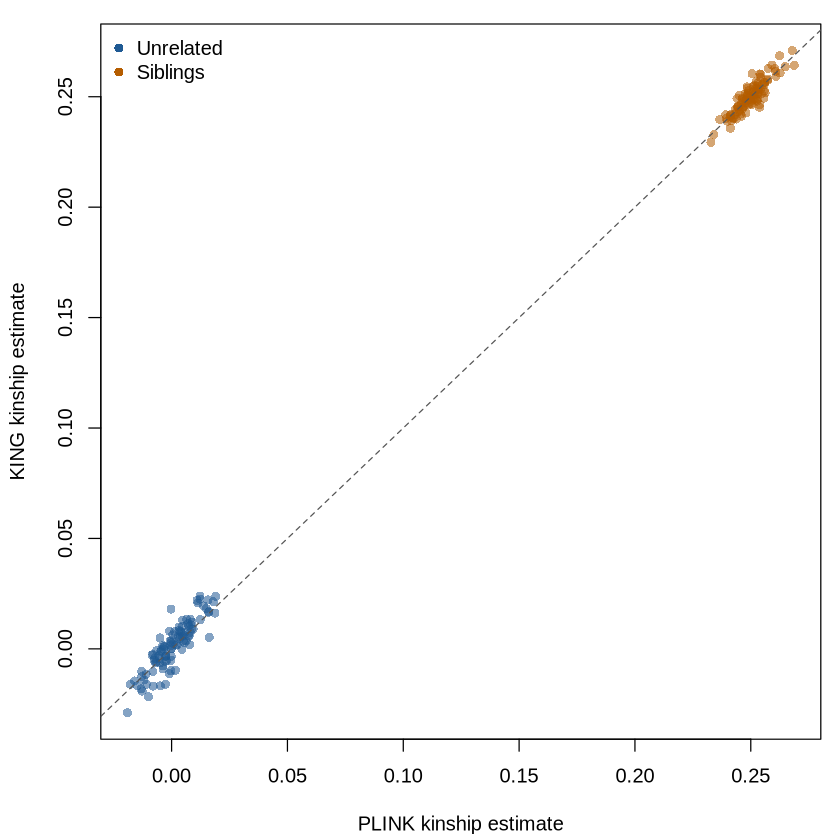

Why a local HMM is unnecessary here¶

A single marker cannot identify local IBD because the same genotype may arise by chance. Linked markers and an HMM resolve that local state.

Genome-wide kinship is an average. It does not require the position of each shared segment. Across many approximately independent markers, chance IBS approaches its expected baseline. The excess estimates average IBD.

Paper2Agent¶

We discussed KING in class. You may use Paper2Agent to explore the original paper.

What to remember¶

Concept and intuition. At one marker, IBS does not identify IBD. Across many markers, chance matches average out.
Insight behind the approach. PLINK estimates the full IBD mixture from IBS counts. KING estimates kinship directly from genotype differences scaled by pair heterozygosity.
Connection. In a homogeneous HWE population with many independent markers, both estimate $\phi=Z_1/4+Z_2/2$ .

Sources¶

Pritchard, An Owner’s Guide to the Human Genome, the linkage material in Chapters 4.1--4.2 and review Chapter 2.3. Book page
Gorroochurn, Notes on Population Genetics, Sections 7.2--7.3.
Purcell et al. (2007), PLINK. DOI
Manichaikul et al. (2010), KING. Paper
The simulation is an original course example. It uses 100 unrelated pairs, 100 sibling pairs, 5,000 independent SNPs, allele frequencies sampled uniformly from 0.10 to 0.50, and seed 8149.

References¶

Purcell, S., Neale, B., Todd-Brown, K., Thomas, L., Ferreira, M. A. R., Bender, D., Maller, J., Sklar, P., de Bakker, P. I. W., Daly, M. J., & Sham, P. C. (2007). PLINK: A Tool Set for Whole-Genome Association and Population-Based Linkage Analyses. The American Journal of Human Genetics, 81(3), 559–575. 10.1086/519795