Linkage, recombination, and LOD scores

We ask one question. Do a DNA marker and a disease allele travel together through a family more often than independent assortment predicts?

This is a simplified parametric linkage example. We treat the disease-bearing chromosome and marker phase as known; a full pedigree model also specifies disease-allele frequency and penetrance.

Start from first principles¶

A meiosis transmits one parental chromosome segment.
A marker near the disease allele usually stays on the same transmitted segment.
The recombination fraction $\theta$ is the probability that recombination separates the two loci in an informative meiosis.
Unlinked loci have $\theta=1/2$ .
A recombinant also marks a boundary for the chromosome region that can contain the disease allele.

This worked example connects dominant inheritance, haplotypes, linkage, co-segregation, and recombination with likelihood ratios and LOD scores.

1. Each meiosis gives evidence about $\theta$ ¶

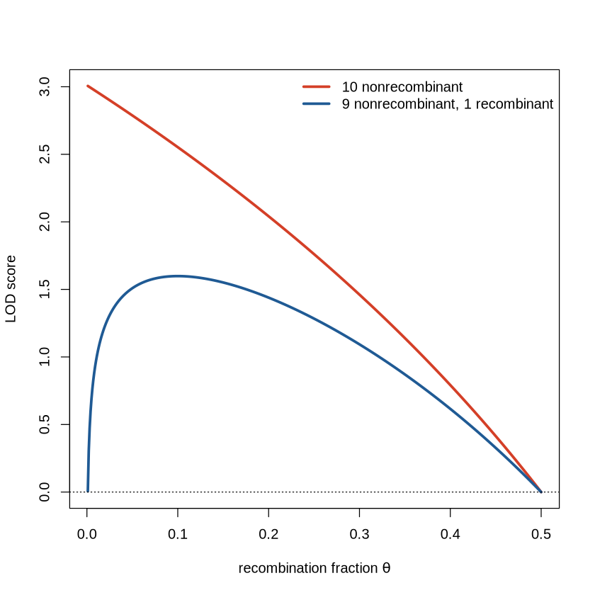
Suppose marker phase is known. Among informative meioses, let $n_N$ be the number of nonrecombinant transmissions and $n_R$ the number of recombinant transmissions. Under the simplest linkage model,

L(\theta)=(1-\theta)^{n_N}\theta^{n_R},\qquad 0\leq\theta\leq\frac12.

(1)

The unlinked model fixes $\theta=1/2$ . The LOD score compares the two models:

\operatorname{LOD}(\theta) =\log_{10}\frac{L(\theta)}{L(1/2)}.

(2)

The maximum-likelihood estimate is $\widehat\theta=n_R/(n_N+n_R)$ when that value is at most $1/2$ .

lod_score <- function(theta, nonrecombinant, recombinant) {
  if (theta < 0 || theta > 0.5) stop("theta must be between 0 and 0.5")
  n <- nonrecombinant + recombinant
  linked <- (1 - theta)^nonrecombinant * theta^recombinant
  unlinked <- 0.5^n
  log10(linked / unlinked)
}

fit_linkage <- function(nonrecombinant, recombinant) {
  n <- nonrecombinant + recombinant
  theta_hat <- min(recombinant / n, 0.5)
  data.frame(
    nonrecombinant = nonrecombinant,
    recombinant = recombinant,
    theta_hat = theta_hat,
    max_LOD = lod_score(theta_hat, nonrecombinant, recombinant)
  )
}

comparison <- rbind(
  fit_linkage(nonrecombinant = 10, recombinant = 0),
  fit_linkage(nonrecombinant = 9, recombinant = 1)
)
comparison

stopifnot(abs(lod_score(0.5, 10, 0)) < 1e-12)
stopifnot(abs(lod_score(0, 10, 0) - 10 * log10(2)) < 1e-12)

theta_grid <- seq(0.001, 0.5, length.out = 500)
lod_no_recombinant <- vapply(
  theta_grid, lod_score, numeric(1), nonrecombinant = 10, recombinant = 0
)
lod_one_recombinant <- vapply(
  theta_grid, lod_score, numeric(1), nonrecombinant = 9, recombinant = 1
)

plot(
  theta_grid, lod_no_recombinant,
  type = "l", lwd = 3, col = "#D43F27",
  xlab = expression("recombination fraction " * theta),
  ylab = "LOD score"
)
lines(theta_grid, lod_one_recombinant, lwd = 3, col = "#1F5A94")
abline(h = 0, lty = 3)
legend(
  "topright",
  legend = c("10 nonrecombinant", "9 nonrecombinant, 1 recombinant"),
  col = c("#D43F27", "#1F5A94"), lwd = 3, bty = "n"
)

2. Independent meioses add evidence¶

For independent meioses, likelihoods multiply. A logarithm turns that product into a sum:

\frac{L_{\mathrm{all}}(\theta)}{L_{\mathrm{all}}(1/2)} =\prod_j \frac{L_j(\theta)}{L_j(1/2)}, \qquad \operatorname{LOD}_{\mathrm{all}}(\theta)=\sum_j\operatorname{LOD}_j(\theta).

(3)

This is the methodological insight. Each informative transmission contributes evidence, and the LOD score keeps a running total on the log scale.

theta <- 0
lod_per_nonrecombinant <- log10((1 - theta) / 0.5)
lod_sum <- sum(rep(lod_per_nonrecombinant, 10))
lod_joint <- lod_score(theta, nonrecombinant = 10, recombinant = 0)

data.frame(
  contribution_per_meiosis = lod_per_nonrecombinant,
  sum_of_contributions = lod_sum,
  joint_LOD = lod_joint
)

stopifnot(abs(lod_sum - lod_joint) < 1e-12)

3. Recombinants also narrow the chromosome region¶

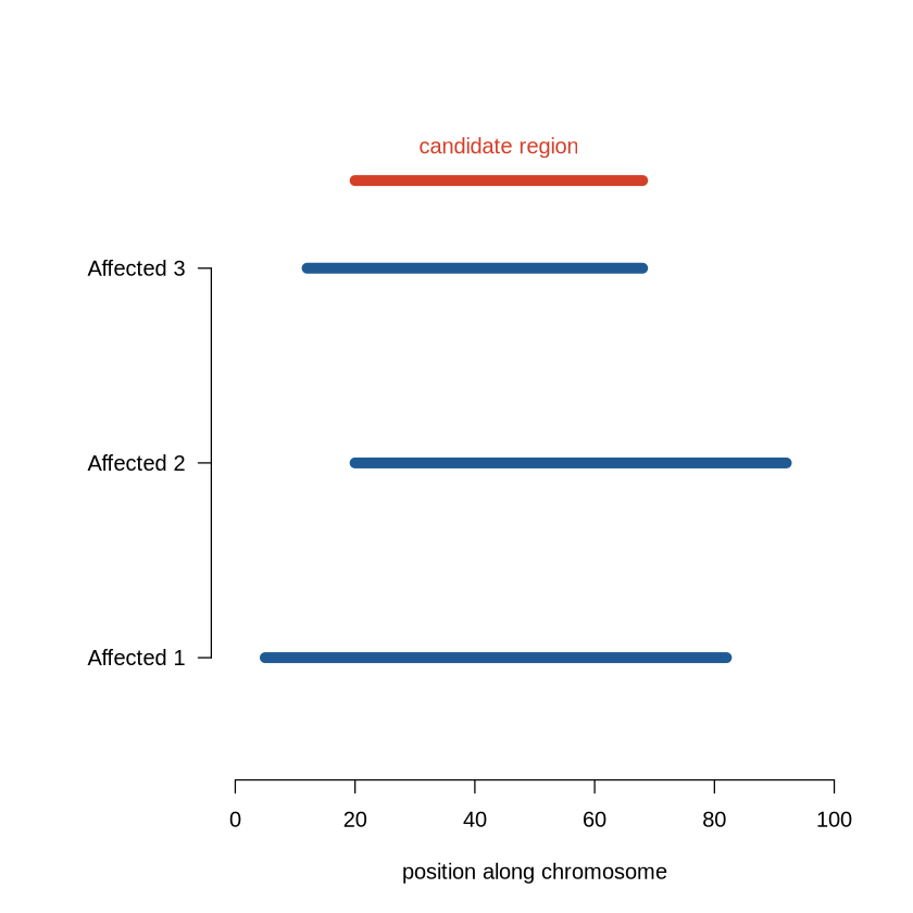
The LOD score asks whether a marker is linked to disease. Recombinant chromosomes tell us where linkage must end. In the toy family below, each affected relative carries part of the disease-associated haplotype. The overlap is the candidate region.

The positions are illustrative, not the original Huntington’s disease coordinates.

shared_segment <- data.frame(
  relative = c("Affected 1", "Affected 2", "Affected 3"),
  left = c(5, 20, 12),
  right = c(82, 92, 68)
)

candidate_left <- max(shared_segment$left)
candidate_right <- min(shared_segment$right)

old_par <- par(mar = c(5, 8, 4, 2) + 0.1)
plot(
  c(0, 100), c(0.5, 3.7), type = "n", axes = FALSE,
  xlab = "position along chromosome", ylab = ""
)
axis(1)
axis(2, at = 1:3, labels = shared_segment$relative, las = 1)
for (i in seq_len(nrow(shared_segment))) {
  segments(
    shared_segment$left[i], i, shared_segment$right[i], i,
    lwd = 8, col = "#1F5A94"
  )
}
segments(candidate_left, 3.45, candidate_right, 3.45, lwd = 8, col = "#D43F27")
text(
  mean(c(candidate_left, candidate_right)), 3.62,
  labels = "candidate region", col = "#D43F27"
)

data.frame(candidate_left = candidate_left, candidate_right = candidate_right)
stopifnot(candidate_left < candidate_right)
invisible(par(old_par))

What to remember¶

Concept and intuition. Nearby loci tend to travel together because few recombination events occur between them.
Methodological insight. Likelihood ratios multiply across independent meioses. LOD scores add the same evidence on the log scale.
Worked example. Ten nonrecombinant meioses give a LOD score of $10\log_{10}2=3.01$ . Recombinants lower the evidence for tight linkage and set candidate-region boundaries.

The calculation assumes known marker phase, a correct inheritance model, and informative meioses. Incomplete penetrance, locus heterogeneity, or pedigree error requires a richer likelihood.

Source record and further detail¶

Pritchard, An Owner’s Guide to the Human Genome, Chapter 4.1 for the Huntington pedigree and Chapter 2.3 for linkage and recombination.
Pritchard, Chapter 4.2, for positional cloning and major-effect mutations.
Gusella et al. (1983), A polymorphic DNA marker genetically linked to Huntington’s disease.
The LOD calculations and candidate-region positions in this notebook are original teaching examples. The exact controls are $\operatorname{LOD}(1/2)=0$ and equality between the joint LOD and the sum of per-meiosis contributions.