DENTIST: Summary Statistics QC via LD-Based Imputation

Overview

DENTIST (Detecting Errors iN analyses of summary staTISTics) performs quality control of GWAS summary statistics by iteratively imputing z-scores using linkage disequilibrium (LD) from a reference panel. Variants whose observed z-scores deviate significantly from their LD-imputed values are flagged as outliers.

The pecotmr package provides a pure R implementation of DENTIST that can be used in two ways:

File-based input via dentist_from_files() — takes PLINK binary files and a summary statistics file, matching the interface of the original DENTIST C++ binary.
Direct input via dentist_single_window() — takes z-scores and an LD matrix (or genotype matrix) directly, suitable for integration into analysis pipelines.

We also demonstrate how the alternative SLALOM + RAISS pipeline achieves comparable QC and imputation on the same data, giving users two complementary approaches for summary statistics quality control.

library(pecotmr)
library(vroom)

Toy Data

We use a toy dataset on chromosome 22 distributed with the package under inst/extdata/. The full dataset has 17,421 variants and 165 reference panel individuals.

# Locate package data
# system.file() finds files within installed packages;
# during development, use the inst/extdata path directly
extdata_dir <- system.file("extdata", package = "pecotmr")
if (extdata_dir == "" || !file.exists(file.path(extdata_dir, "toy_ref.bed"))) {
  # Fallback for development: look relative to the package source root
  extdata_dir <- file.path(getwd(), "..", "inst", "extdata")
  if (!file.exists(file.path(extdata_dir, "toy_ref.bed"))) {
    extdata_dir <- file.path(getwd(), "inst", "extdata")
  }
}
bfile <- file.path(extdata_dir, "toy_ref")
sumstat_gz <- file.path(extdata_dir, "toy_summary.txt.gz")

# Load summary statistics (DENTIST format: SNP A1 A2 freq beta se p N)
sumstat <- as.data.frame(vroom(sumstat_gz, show_col_types = FALSE))
cat(sprintf("Full dataset: %d variants\n", nrow(sumstat)))

## Full dataset: 17421 variants

head(sumstat, 3)

##          SNP A1 A2   freq      beta       se         p     N
## 1 rs11089128  G  A 0.0804 -0.008047 0.014364 0.5753294 10000
## 2  rs7288972  C  T 0.1741 -0.025328 0.028768 0.3786304 10000
## 3 rs11167319  G  T 0.1339 -0.001455 0.023300 0.9502074 10000

Case 1: File-Based DENTIST with Windowed QC

The dentist_from_files() function mirrors the interface of the DENTIST C++ binary. It takes a summary statistics file path and a PLINK bfile prefix, then internally handles allele alignment, LD computation, and windowed imputation.

DENTIST supports two windowing strategies:

Distance mode (window_mode = "distance", default): windows span a fixed physical distance (window_size bp). This is the original DENTIST algorithm (--wind-dist).
Count mode (window_mode = "count"): windows contain a fixed number of variants (min_dim). This corresponds to the C++ --wind flag.

Here we demonstrate count mode on the full dataset, which avoids the “<2000 variants” warning that distance mode produces on regions with sparse variant density.

Run with `min_dim = 2000`

# Write the full summary statistics to a temp file for dentist_from_files
full_sumstat <- tempfile(fileext = ".txt")
readr::write_tsv(sumstat, full_sumstat)

# Run DENTIST with count-based windowing: 2000 variants per window
result_2000 <- dentist_from_files(
  gwas_summary = full_sumstat,
  bfile        = bfile,
  nSample      = NULL,
  window_mode  = "count",
  min_dim      = 2000,
  nIter        = 8,
  pValueThreshold = 5.0369e-08,
  propSVD      = 0.4,
  duprThreshold = 0.99,
  verbose      = FALSE
)

## Rows: 17421 Columns: 6
## ── Column specification ────────────────────────────────────────────────────────
## Delimiter: "\t"
## chr (3): X2, X5, X6
## dbl (3): X1, X3, X4
## 
## ℹ Use `spec()` to retrieve the full column specification for this data.
## ℹ Specify the column types or set `show_col_types = FALSE` to quiet this message.
## 514 duplicated variants out of a total of 2000 were found at r threshold of 0.995
## 
## 595 duplicated variants out of a total of 2000 were found at r threshold of 0.995
## 
## 538 duplicated variants out of a total of 2000 were found at r threshold of 0.995
## 
## 510 duplicated variants out of a total of 2000 were found at r threshold of 0.995
## 
## 403 duplicated variants out of a total of 2000 were found at r threshold of 0.995
## 
## 467 duplicated variants out of a total of 2000 were found at r threshold of 0.995
## 
## 514 duplicated variants out of a total of 2000 were found at r threshold of 0.995
## 
## 519 duplicated variants out of a total of 2000 were found at r threshold of 0.995
## 
## 578 duplicated variants out of a total of 2000 were found at r threshold of 0.995
## 
## 532 duplicated variants out of a total of 2000 were found at r threshold of 0.995
## 
## 569 duplicated variants out of a total of 2000 were found at r threshold of 0.995
## 
## 575 duplicated variants out of a total of 2000 were found at r threshold of 0.995
## 
## 418 duplicated variants out of a total of 2000 were found at r threshold of 0.995
## 
## 357 duplicated variants out of a total of 2000 were found at r threshold of 0.995
## 
## 395 duplicated variants out of a total of 2000 were found at r threshold of 0.995
## 
## 424 duplicated variants out of a total of 2421 were found at r threshold of 0.995

cat(sprintf("min_dim = 2000: %d variants, %d outliers (%.1f%%)\n",
            nrow(result_2000$result),
            sum(result_2000$result$outlier),
            100 * mean(result_2000$result$outlier)))

## min_dim = 2000: 17421 variants, 1430 outliers (8.2%)

Run with `min_dim = 6000`

# Run DENTIST with larger windows: 6000 variants per window
result_6000 <- dentist_from_files(
  gwas_summary = full_sumstat,
  bfile        = bfile,
  nSample      = NULL,
  window_mode  = "count",
  min_dim      = 6000,
  nIter        = 8,
  pValueThreshold = 5.0369e-08,
  propSVD      = 0.4,
  duprThreshold = 0.99,
  verbose      = FALSE
)

## Rows: 17421 Columns: 6
## ── Column specification ────────────────────────────────────────────────────────
## Delimiter: "\t"
## chr (3): X2, X5, X6
## dbl (3): X1, X3, X4
## 
## ℹ Use `spec()` to retrieve the full column specification for this data.
## ℹ Specify the column types or set `show_col_types = FALSE` to quiet this message.
## 1456 duplicated variants out of a total of 6000 were found at r threshold of 0.995
## 
## 1499 duplicated variants out of a total of 6000 were found at r threshold of 0.995
## 
## 1663 duplicated variants out of a total of 6000 were found at r threshold of 0.995
## 
## 1889 duplicated variants out of a total of 8421 were found at r threshold of 0.995

cat(sprintf("min_dim = 6000: %d variants, %d outliers (%.1f%%)\n",
            nrow(result_6000$result),
            sum(result_6000$result$outlier),
            100 * mean(result_6000$result$outlier)))

## min_dim = 6000: 17421 variants, 266 outliers (1.5%)

Sensitivity to Window Size

cat("=== DENTIST Outlier Detection by Window Size ===\n\n")

## === DENTIST Outlier Detection by Window Size ===

cat(sprintf("  min_dim = 2000:  %d outliers (%.1f%%)\n",
            sum(result_2000$result$outlier), 100 * mean(result_2000$result$outlier)))

##   min_dim = 2000:  1430 outliers (8.2%)

cat(sprintf("  min_dim = 6000:  %d outliers (%.1f%%)\n",
            sum(result_6000$result$outlier), 100 * mean(result_6000$result$outlier)))

##   min_dim = 6000:  266 outliers (1.5%)

cat("  min_dim = 20000: 97 outliers (0.6%) [not run here; ~4 min compute time]\n")

##   min_dim = 20000: 97 outliers (0.6%) [not run here; ~4 min compute time]

The number of detected outliers varies substantially with window size: smaller windows detect more outliers (8.2% at 2000) while larger windows detect far fewer (1.5% at 6000, 0.6% at 20000). We do not run min_dim = 20000 in this vignette because it takes approximately 4 minutes to compute on this dataset.

This sensitivity to window size means that DENTIST outlier counts should be interpreted with caution. The windowed approach inherently couples QC results to the choice of window parameters, which is a known limitation. For a more robust QC approach, consider using SLALOM (demonstrated below), which does not depend on window size parameters.

The dentist_from_files() return value is a list with three components:

result — data frame with outlier detection results (one row per input variant)
sum_stat — aligned summary statistics after allele QC
LD_mat — the LD correlation matrix used for imputation

Case 2: Single-Window DENTIST vs SLALOM + RAISS

For pipeline integration, dentist_single_window() accepts z-scores and an LD matrix directly. We compare this with the SLALOM + RAISS pipeline, which uses a different approach to achieve the same goal: identifying problematic variants and imputing corrected z-scores.

DENTIST performs iterative SVD-truncated imputation: it imputes all z-scores from LD, flags outliers based on the discrepancy statistic (z_obs - z_imp)^2 / (1 - r^2), removes flagged variants, and repeats.

SLALOM computes the DENTIST-S statistic relative to the lead variant to flag outliers among variants in high LD. RAISS then imputes z-scores for a given set of variants using LD-based regression from the remaining variants.

Prepare aligned data

We subset to a smaller region for the single-window comparison, since dentist_single_window() operates on a single LD matrix in memory.

# Load reference panel variant info
bim <- as.data.frame(vroom(paste0(bfile, ".bim"), col_names = c("chrom", "variant_id", "gd", "pos", "A1", "A2"),
                           show_col_types = FALSE))

# Select ~500 variants from a contiguous region for fast execution
region_start <- bim$pos[1]
region_end   <- region_start + 2e6
region_snps  <- bim$variant_id[bim$pos >= region_start & bim$pos <= region_end]
cat(sprintf("Selected %d variants in %.1f Mb region (pos %s - %s)\n",
            length(region_snps),
            (region_end - region_start) / 1e6,
            format(region_start, big.mark = ","),
            format(region_end, big.mark = ",")))

## Selected 608 variants in 2.0 Mb region (pos 14,560,203 - 16,560,203)

# Subset summary statistics to the selected region and run DENTIST
sumstat_sub <- sumstat[sumstat$SNP %in% region_snps, ]
sub_sumstat <- tempfile(fileext = ".txt")
readr::write_tsv(sumstat_sub, sub_sumstat)
cat(sprintf("Subset: %d variants in summary stats\n", nrow(sumstat_sub)))

## Subset: 608 variants in summary stats

# Run DENTIST on the subset (count mode, small windows for toy data)
result_files <- dentist_from_files(
  gwas_summary = sub_sumstat,
  bfile        = bfile,
  nSample      = NULL,
  window_mode  = "count",
  min_dim      = 500,
  nIter        = 8,
  pValueThreshold = 5.0369e-08,
  propSVD      = 0.4,
  duprThreshold = 0.99,
  verbose      = FALSE
)

## Rows: 17421 Columns: 6
## ── Column specification ────────────────────────────────────────────────────────
## Delimiter: "\t"
## chr (3): X2, X5, X6
## dbl (3): X1, X3, X4
## 
## ℹ Use `spec()` to retrieve the full column specification for this data.
## ℹ Specify the column types or set `show_col_types = FALSE` to quiet this message.
## 98 duplicated variants out of a total of 608 were found at r threshold of 0.995

# Use the aligned data from dentist_from_files for consistency
# This ensures allele QC has already been applied
aligned_sumstat <- result_files$sum_stat
LD_mat <- result_files$LD_mat
n_samples <- nrow(vroom(paste0(bfile, ".fam"), col_names = FALSE, show_col_types = FALSE))

z_scores <- aligned_sumstat$z
n_snps <- length(z_scores)
cat(sprintf("Aligned data: %d variants, %d reference samples\n", n_snps, n_samples))

## Aligned data: 608 variants, 165 reference samples

# Build a position-sorted variant info data frame for RAISS
bim_full <- as.data.frame(vroom(paste0(bfile, ".bim"), col_names = c("chrom", "variant_id", "gd", "pos", "A1", "A2"),
                              show_col_types = FALSE))
bim_aligned <- bim_full[match(aligned_sumstat$SNP, bim_full$variant_id), ]

# Sort everything by position (required by RAISS)
pos_order <- order(bim_aligned$pos)
ref_panel_df <- data.frame(
  chrom      = bim_aligned$chrom[pos_order],
  pos        = bim_aligned$pos[pos_order],
  variant_id = bim_aligned$variant_id[pos_order],
  A1         = bim_aligned$A1[pos_order],
  A2         = bim_aligned$A2[pos_order],
  stringsAsFactors = FALSE
)
z_sorted <- z_scores[pos_order]
LD_sorted <- LD_mat[pos_order, pos_order]

Run DENTIST (single-window)

dentist_sw <- dentist_single_window(
  zScore   = z_sorted,
  R        = LD_sorted,
  nSample  = n_samples,
  pValueThreshold = 5.0369e-08,
  propSVD  = 0.4,
  nIter    = 8,
  duprThreshold = 0.99
)

## 98 duplicated variants out of a total of 608 were found at r threshold of 0.995

cat(sprintf("DENTIST single-window: %d variants, %d outliers (%.1f%%)\n",
            nrow(dentist_sw),
            sum(dentist_sw$outlier),
            100 * mean(dentist_sw$outlier)))

## DENTIST single-window: 608 variants, 119 outliers (19.6%)

Run SLALOM (QC)

SLALOM uses Approximate Bayes Factors for fine-mapping and the DENTIST-S statistic for outlier detection. It identifies variants whose z-scores are inconsistent with the lead variant’s LD pattern. Note that SLALOM focuses on variants in high LD with the lead variant (r^2 > threshold), so it typically flags fewer outliers than DENTIST’s genome-wide iterative approach.

slalom_result <- slalom(
  zScore = z_sorted,
  R      = LD_sorted,
  nlog10p_dentist_s_threshold = 4.0,
  r2_threshold = 0.6
)

# Replace NA outlier flags with FALSE (NAs arise from division by zero
# when a variant is in perfect LD with the lead variant)
slalom_outliers <- slalom_result$data$outliers
slalom_outliers[is.na(slalom_outliers)] <- FALSE
cat(sprintf("SLALOM: %d outliers out of %d variants (%.1f%%)\n",
            sum(slalom_outliers),
            length(slalom_outliers),
            100 * mean(slalom_outliers)))

## SLALOM: 1 outliers out of 608 variants (0.2%)

cat(sprintf("SLALOM lead variant PIP: %.4f\n", slalom_result$summary$max_pip))

## SLALOM lead variant PIP: 0.0047

cat(sprintf("95%% credible set size: %d\n", length(slalom_result$summary$cs_95)))

## 95% credible set size: 577

Run RAISS on SLALOM-flagged outliers

RAISS imputes z-scores for “unknown” variants using LD with “known” variants. First, we use SLALOM’s outlier flags to define which variants to re-impute — this is the natural SLALOM+RAISS pipeline.

# Helper: run RAISS given a set of outlier flags
run_raiss_on_outliers <- function(outlier_flags, z_vec, ref_df, LD_mat) {
  known_idx <- which(!outlier_flags)
  known_df <- data.frame(
    chrom      = ref_df$chrom[known_idx],
    pos        = ref_df$pos[known_idx],
    variant_id = ref_df$variant_id[known_idx],
    A1         = ref_df$A1[known_idx],
    A2         = ref_df$A2[known_idx],
    z          = z_vec[known_idx],
    stringsAsFactors = FALSE
  )
  result <- raiss(
    ref_panel     = ref_df,
    known_zscores = known_df,
    LD_matrix     = LD_mat,
    lamb = 0.01, rcond = 0.01,
    R2_threshold = 0.6, minimum_ld = 5, verbose = FALSE
  )
  # Build combined z-score vector
  combined_z <- z_vec
  if (!is.null(result) && !is.null(result$result_nofilter)) {
    raiss_df <- result$result_nofilter
    for (i in which(outlier_flags)) {
      vid <- ref_df$variant_id[i]
      ri <- which(raiss_df$variant_id == vid)
      if (length(ri) == 1 && !is.na(raiss_df$z[ri])) {
        combined_z[i] <- raiss_df$z[ri]
      }
    }
  }
  return(list(z = combined_z, raiss_result = result))
}

cat(sprintf("SLALOM+RAISS: using %d SLALOM outliers as variants to impute\n",
            sum(slalom_outliers)))

## SLALOM+RAISS: using 1 SLALOM outliers as variants to impute

slalom_raiss <- run_raiss_on_outliers(slalom_outliers, z_sorted, ref_panel_df, LD_sorted)

Run RAISS on DENTIST-flagged outliers

Next, we use DENTIST’s outlier flags with RAISS imputation. This lets us directly compare how DENTIST and RAISS impute the same set of variants.

dentist_outlier_flags <- dentist_sw$outlier
cat(sprintf("DENTIST+RAISS: using %d DENTIST outliers as variants to impute\n",
            sum(dentist_outlier_flags)))

## DENTIST+RAISS: using 119 DENTIST outliers as variants to impute

dentist_raiss <- run_raiss_on_outliers(dentist_outlier_flags, z_sorted, ref_panel_df, LD_sorted)

Compare All Three Approaches

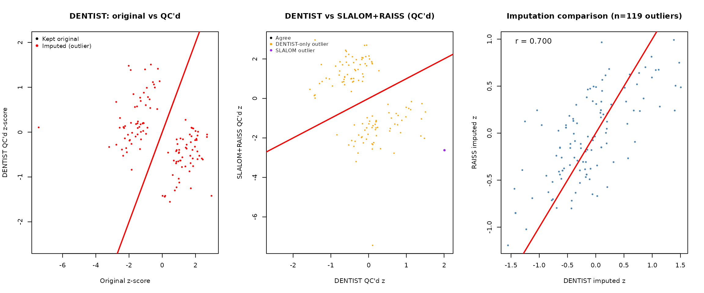
We now have three sets of z-scores:

DENTIST: iterative SVD-truncated imputation (imputes all variants)
SLALOM+RAISS: SLALOM flags outliers, RAISS imputes those
DENTIST+RAISS: DENTIST flags outliers, RAISS imputes those

# Build "QC'd z-scores" for each pipeline:
# Each keeps original z for non-outliers, replaces outlier z with imputed values

# DENTIST QC'd: original z for non-outliers, DENTIST imputed z for outliers
dentist_qc_z <- z_sorted
dentist_qc_z[dentist_outlier_flags] <- dentist_sw$imputed_z[dentist_outlier_flags]

# SLALOM+RAISS QC'd: original z for non-outliers, RAISS imputed z for SLALOM outliers
slalom_raiss_z <- slalom_raiss$z

# DENTIST-flags+RAISS QC'd: original z for non-outliers, RAISS imputed z for DENTIST outliers
dentist_raiss_z <- dentist_raiss$z

cat("=== Three-Way Comparison ===\n")

## === Three-Way Comparison ===

cat(sprintf("Total variants: %d\n\n", n_snps))

## Total variants: 608

# Outlier counts
cat("Outlier detection:\n")

## Outlier detection:

cat(sprintf("  DENTIST outliers: %d (%.1f%%)\n",
            sum(dentist_outlier_flags), 100 * mean(dentist_outlier_flags)))

##   DENTIST outliers: 119 (19.6%)

cat(sprintf("  SLALOM outliers:  %d (%.1f%%)\n",
            sum(slalom_outliers), 100 * mean(slalom_outliers)))

##   SLALOM outliers:  1 (0.2%)

overlap <- sum(dentist_outlier_flags & slalom_outliers)
cat(sprintf("  Overlap:          %d\n\n", overlap))

##   Overlap:          0

# Correlation between QC'd z-score vectors
cat("QC'd z-score correlations (all variants):\n")

## QC'd z-score correlations (all variants):

cat(sprintf("  DENTIST vs SLALOM+RAISS:       %.4f\n", cor(dentist_qc_z, slalom_raiss_z)))

##   DENTIST vs SLALOM+RAISS:       0.4917

cat(sprintf("  DENTIST vs DENTIST+RAISS:      %.4f\n", cor(dentist_qc_z, dentist_raiss_z)))

##   DENTIST vs DENTIST+RAISS:      0.9622

cat(sprintf("  SLALOM+RAISS vs DENTIST+RAISS: %.4f\n\n",
            cor(slalom_raiss_z, dentist_raiss_z)))

##   SLALOM+RAISS vs DENTIST+RAISS: 0.5530

# Focus on DENTIST-flagged outliers (where imputation matters most)
if (sum(dentist_outlier_flags) > 1) {
  d_out <- dentist_outlier_flags
  cat("On DENTIST-flagged outlier variants:\n")
  cat(sprintf("  DENTIST imputed vs RAISS imputed: r = %.4f\n",
              cor(dentist_sw$imputed_z[d_out], dentist_raiss_z[d_out])))
  cat(sprintf("  Mean |diff|: %.3f, Max |diff|: %.3f\n",
              mean(abs(dentist_sw$imputed_z[d_out] - dentist_raiss_z[d_out])),
              max(abs(dentist_sw$imputed_z[d_out] - dentist_raiss_z[d_out]))))
}

## On DENTIST-flagged outlier variants:
##   DENTIST imputed vs RAISS imputed: r = 0.7002
##   Mean |diff|: 0.380, Max |diff|: 1.377

par(mfrow = c(1, 3))

# Panel 1: DENTIST QC'd z vs original
plot(z_sorted, dentist_qc_z, pch = 16, cex = 0.4, col = rgb(0, 0, 0, 0.3),
     xlab = "Original z-score", ylab = "DENTIST QC'd z-score",
     main = "DENTIST: original vs QC'd")
abline(0, 1, col = "red", lwd = 2)
if (sum(dentist_outlier_flags) > 0) {
  points(z_sorted[dentist_outlier_flags], dentist_qc_z[dentist_outlier_flags],
         pch = 16, cex = 0.6, col = "red")
  legend("topleft", legend = c("Kept original", "Imputed (outlier)"),
         col = c("black", "red"), pch = 16, bty = "n", cex = 0.9)
}

# Panel 2: DENTIST QC'd vs SLALOM+RAISS QC'd
plot(dentist_qc_z, slalom_raiss_z, pch = 16, cex = 0.4, col = rgb(0, 0, 0, 0.3),
     xlab = "DENTIST QC'd z", ylab = "SLALOM+RAISS QC'd z",
     main = "DENTIST vs SLALOM+RAISS (QC'd)")
abline(0, 1, col = "red", lwd = 2)
# Highlight DENTIST outliers (where DENTIST replaced z but SLALOM did not)
dentist_only <- dentist_outlier_flags & !slalom_outliers
if (sum(dentist_only) > 0) {
  points(dentist_qc_z[dentist_only], slalom_raiss_z[dentist_only],
         pch = 16, cex = 0.5, col = "orange")
}
if (sum(slalom_outliers) > 0) {
  points(dentist_qc_z[slalom_outliers], slalom_raiss_z[slalom_outliers],
         pch = 16, cex = 0.8, col = "purple")
}
legend("topleft",
       legend = c("Agree", "DENTIST-only outlier", "SLALOM outlier"),
       col = c("black", "orange", "purple"), pch = 16, bty = "n", cex = 0.8)

# Panel 3: DENTIST imputed vs RAISS imputed (on DENTIST outliers)
if (sum(dentist_outlier_flags) > 1) {
  d_out <- dentist_outlier_flags
  plot(dentist_sw$imputed_z[d_out], dentist_raiss_z[d_out],
       pch = 16, cex = 0.6, col = "steelblue",
       xlab = "DENTIST imputed z", ylab = "RAISS imputed z",
       main = sprintf("Imputation comparison (n=%d outliers)",
                       sum(d_out)))
  abline(0, 1, col = "red", lwd = 2)
  legend("topleft",
         legend = sprintf("r = %.3f",
                          cor(dentist_sw$imputed_z[d_out], dentist_raiss_z[d_out])),
         bty = "n", cex = 1.2)
} else {
  plot.new()
  text(0.5, 0.5, "Too few outliers\nfor comparison", cex = 1.2)
}

Summary

The pecotmr package provides two complementary approaches for GWAS summary statistics QC:

DENTIST-based (dentist_from_files / dentist_single_window):

Iterative SVD-truncated imputation across the full LD structure
Flags outliers via chi-squared test on (z_obs - z_imp)^2 / (1 - r^2)
Produces imputed z-scores for all variants simultaneously
Results are sensitive to window size (as shown in Case 1), which is a known limitation

SLALOM + RAISS-based (slalom + raiss):

SLALOM identifies outliers via the DENTIST-S statistic relative to the lead variant
RAISS imputes outlier z-scores using LD regression from non-outlier variants
Provides per-variant imputation quality (R^2) and LD scores for filtering
Does not depend on window size parameters, making results more stable

Both methods require an LD reference panel and perform allele QC as a preprocessing step. Given the sensitivity of DENTIST to window size parameters, SLALOM is the recommended default QC method in pecotmr (set via qc_method = "slalom" in pipeline functions). SLALOM+RAISS integrates naturally with fine-mapping workflows where posterior inclusion probabilities and credible sets are also needed.

sessionInfo()

## R version 4.4.3 (2025-02-28)
## Platform: x86_64-conda-linux-gnu
## Running under: Ubuntu 24.04.4 LTS
## 
## Matrix products: default
## BLAS/LAPACK: /home/runner/work/pecotmr/pecotmr/.pixi/envs/r44/lib/libopenblasp-r0.3.32.so;  LAPACK version 3.12.0
## 
## locale:
##  [1] LC_CTYPE=C.UTF-8       LC_NUMERIC=C           LC_TIME=C.UTF-8       
##  [4] LC_COLLATE=C.UTF-8     LC_MONETARY=C.UTF-8    LC_MESSAGES=C.UTF-8   
##  [7] LC_PAPER=C.UTF-8       LC_NAME=C              LC_ADDRESS=C          
## [10] LC_TELEPHONE=C         LC_MEASUREMENT=C.UTF-8 LC_IDENTIFICATION=C   
## 
## time zone: Etc/UTC
## tzcode source: system (glibc)
## 
## attached base packages:
## [1] stats     graphics  grDevices utils     datasets  methods   base     
## 
## other attached packages:
## [1] vroom_1.7.1   pecotmr_0.5.0
## 
## loaded via a namespace (and not attached):
##   [1] tidyselect_1.2.1      viridisLite_0.4.3     bigsnpr_1.12.21      
##   [4] dplyr_1.2.1           farver_2.1.2          viridis_0.6.5        
##   [7] S7_0.2.1              fastmap_1.2.0         reshape_0.8.10       
##  [10] bigassertr_0.1.7      flock_0.7             digest_0.6.39        
##  [13] lifecycle_1.0.5       survival_3.8-6        magrittr_2.0.5       
##  [16] compiler_4.4.3        rlang_1.2.0           sass_0.4.10          
##  [19] rngtools_1.5.2        tools_4.4.3           yaml_2.3.12          
##  [22] data.table_1.17.8     knitr_1.51            doRNG_1.8.6.3        
##  [25] htmlwidgets_1.6.4     bit_4.6.0             plyr_1.8.9           
##  [28] RColorBrewer_1.1-3    rmio_0.4.0            coloc_5.2.3          
##  [31] withr_3.0.2           bigsparser_0.7.3      purrr_1.2.1          
##  [34] bigstatsr_1.6.2       BiocGenerics_0.52.0   desc_1.4.3           
##  [37] grid_4.4.3            stats4_4.4.3          susieR_0.15.53       
##  [40] future_1.70.0         ggplot2_4.0.2         MASS_7.3-65          
##  [43] globals_0.19.1        scales_1.4.0          iterators_1.0.14     
##  [46] cli_3.6.5             rmarkdown_2.31        crayon_1.5.3         
##  [49] ragg_1.5.2            generics_0.1.4        RcppParallel_5.1.11-2
##  [52] otel_0.2.0            future.apply_1.20.2   tzdb_0.5.0           
##  [55] cachem_1.1.0          stringr_1.6.0         splines_4.4.3        
##  [58] zlibbioc_1.52.0       parallel_4.4.3        matrixStats_1.5.0    
##  [61] vctrs_0.7.2           Matrix_1.7-5          jsonlite_2.0.0       
##  [64] IRanges_2.40.0        hms_1.1.4             S4Vectors_0.44.0     
##  [67] bit64_4.6.0-1         mixsqp_0.3-54         irlba_2.3.7          
##  [70] listenv_0.10.1        systemfonts_1.3.2     foreach_1.5.2        
##  [73] tidyr_1.3.2           jquerylib_0.1.4       bigparallelr_0.3.2   
##  [76] snpStats_1.56.0       glue_1.8.0            parallelly_1.46.1    
##  [79] pkgdown_2.2.0         codetools_0.2-20      cowplot_1.2.0        
##  [82] stringi_1.8.7         gtable_0.3.6          doFuture_1.2.1       
##  [85] tibble_3.3.1          pillar_1.11.1         furrr_0.4.0          
##  [88] htmltools_0.5.9       R6_2.6.1              zigg_0.0.2           
##  [91] textshaping_1.0.5     doParallel_1.0.17     evaluate_1.0.5       
##  [94] lattice_0.22-9        readr_2.2.0           Rfast_2.1.5.2        
##  [97] bslib_0.10.0          Rcpp_1.1.1            gridExtra_2.3        
## [100] xfun_0.57             fs_1.6.7              pkgconfig_2.0.3

Haochen Sun with Claude Opus 4.6

2026-04-07

Overview

Toy Data

Case 1: File-Based DENTIST with Windowed QC

Run with `min_dim = 2000`

Run with `min_dim = 6000`

Sensitivity to Window Size

Case 2: Single-Window DENTIST vs SLALOM + RAISS

Prepare aligned data

Run DENTIST (single-window)

Run SLALOM (QC)

Run RAISS on SLALOM-flagged outliers

Run RAISS on DENTIST-flagged outliers

Compare All Three Approaches

Summary

DENTIST: Summary Statistics QC via LD-Based Imputation

Haochen Sun with Claude Opus 4.6

2026-04-07

Overview

Toy Data

Case 1: File-Based DENTIST with Windowed QC

Run with min_dim = 2000

Run with min_dim = 6000

Sensitivity to Window Size

Case 2: Single-Window DENTIST vs SLALOM + RAISS

Prepare aligned data

Run DENTIST (single-window)

Run SLALOM (QC)

Run RAISS on SLALOM-flagged outliers

Run RAISS on DENTIST-flagged outliers

Compare All Three Approaches

Summary

Run with `min_dim = 2000`

Run with `min_dim = 6000`