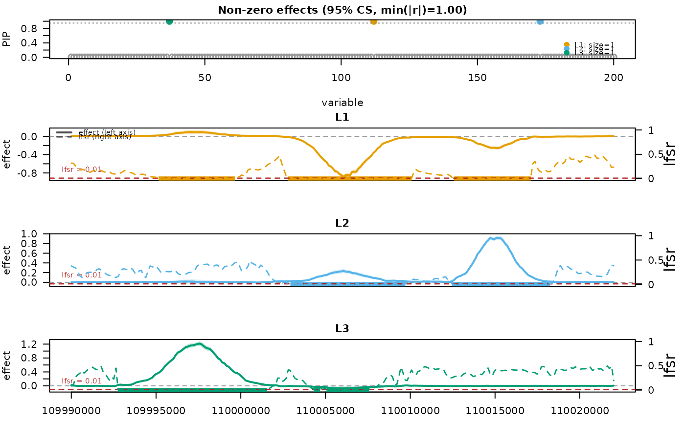
Simulated GTEx-style cis-eQTL example

Simulated cis-eQTL data inspired by published GTEx case studies (AHCYL1, SCD, HSP90AA1, STMN2, ABHD17A): a functional response on 256 gene-body positions, three causal SNPs with localized peak effects at distinct 5', mid-body, and 3' positions. Used by vignette("fsusie_gtex_case_study").

Usage

gtex_example

Format

A list with components

X

n x p genotype matrix (p = 200) sliced from susieR::N3finemapping$X.

Y

n x T log1p-coverage matrix (T = 256).

pos

length-T integer vector of gene-body positions.

causal_snps

integer vector of column indices in X that carry true effects.

causal_betas

length(causal_snps) x T matrix of true per-position effects.

description

free-text description.

Source

Simulated. See data-raw/make_data.R.

Examples

# \donttest{
data(gtex_example)
fit <- fsusie(gtex_example$Y, gtex_example$X,
              pos = gtex_example$pos, L = 15, L_greedy = 5,
              verbose = TRUE)
#> HINT: ncol(Y) is not 2^J or positions are unevenly spaced; interpolated to a regular dyadic grid.
#> iter          ELBO       delta   sigma2      mem      V  extras
#>    1   -205997.7982           -   [0.998, 0.998, 0.999]   0.21 GB  [1.00e+00, 1.00e+00, 1.00e+00, 1.00e+00, 1.00e+00]  pi_null=[1.00, 1.00]
#> iter   2: max|dPIP|=4.80e-06, V=[1.00e+00, 1.00e+00, 1.00e+00, 1.00e+00, 1.00e+00] -- converged [mem: 0.21 GB]
#> [L_greedy] 1 round, greedy_lbf_cutoff=0.100, final L=5
#> round  L     min(lbf)   action
#> 1      5     0.000      saturated
fit_s <- mf_post_smooth(fit, method = "TI")
mfsusie_plot(fit_s)

# }