GTEx-style RNA-seq cis-eQTL fine-mapping
Gao Wang, Anjing Liu and William Denault
Source:vignettes/fsusie_gtex_case_study.Rmd
fsusie_gtex_case_study.RmdThis vignette walks through a GTEx-style cis-eQTL fine-mapping
analysis using fsusie(). The phenotype is RNA-seq read
coverage along a gene body; fsusie() treats it as a single
functional response and returns credible sets of variants that drive
coordinated changes in expression at distinct positions of the gene.
The published case studies (AHCYL1, SCD, HSP90AA1, STMN2, ABHD17A)
all share this shape: a multi-CS fit on log1p-transformed RNA-seq counts
over a cis window. The underlying GTEx individual-level data is
protected and cannot be redistributed with this package, so we
simulate data (gtex_example) that reproduces the multi-CS
structure of those figures and walk through both the standard plot and a
publication-grade genome-browser overlay on this simulated data.
Example dataset
library(mfsusieR)
data(gtex_example)
str(gtex_example, max.level = 1)
#> List of 11
#>  $ X           : num [1:574, 1:200] 0.411 0.411 -0.589 0.411 0.411 ...
#>  $ Y           : num [1:574, 1:256] 3.75 3.97 3.7 3.81 3.89 ...
#>  $ pos         : num [1:256] 1.1e+08 1.1e+08 1.1e+08 1.1e+08 1.1e+08 ...
#>  $ snp_pos     : int [1:200] 109842832 109843862 109846216 109846518 109847130 109847559 109848789 109849391 109849689 109850687 ...
#>  $ chrom       : chr "chr1"
#>  $ gene        : chr "AHCYL1-like"
#>  $ locus       : int [1:2] 109990000 110022000
#>  $ gene_track  :'data.frame':    10 obs. of  9 variables:
#>  $ causal_snps : int [1:3] 37 112 173
#>  $ causal_betas: num [1:3, 1:256] 6.76e-06 -6.22e-37 4.12e-135 1.01e-05 -2.25e-36 ...
#>  $ description : chr "Simulated GTEx-style cis-eQTL example. n = 574, p = 200 SNPs over the susieR::N3finemapping LD scaffold, T = 25"| __truncated__
200 SNPs over a real LD scaffold
(susieR::N3finemapping$X), 256 gene-body positions in a 32
kb window on chr1 (109.99 Mb - 110.02 Mb), three causal SNPs at distinct
positions (5’, mid-body, 3’) with localized peak effects.
Fit
fit <- fsusie(gtex_example$Y, gtex_example$X,
              pos = gtex_example$pos)
#> HINT: ncol(Y) is not 2^J or positions are unevenly spaced; interpolated to a regular dyadic grid.
#> iter          ELBO       delta   sigma2      mem      V  extras
#>    1   -205841.8728           -   [0.998, 0.998, 1.000]   0.82 GB  [1.75e-02, 1.16e-02, 9.48e-03, 1.01e-03, 0 x 1]  pi_null=[0.92, 1.00]
#> iter   2: max|d(alpha,PIP)|=1.60e-01, V=[1.63e-02, 1.50e-02, 9.98e-03, 1.38e-03, 0 x 1] [mem: 0.82 GB]
#> iter   3: max|d(alpha,PIP)|=1.70e-01, V=[1.61e-02, 1.51e-02, 9.99e-03, 1.33e-03, 0 x 1] [mem: 0.82 GB]
#> iter   4: max|d(alpha,PIP)|=1.65e-01, V=[1.60e-02, 1.51e-02, 1.00e-02, 1.22e-03, 0 x 1] [mem: 0.82 GB]
#> iter   5: max|d(alpha,PIP)|=1.56e-01, V=[1.58e-02, 1.51e-02, 1.00e-02, 1.13e-03, 0 x 1] [mem: 0.82 GB]
#> iter   6: max|d(alpha,PIP)|=1.46e-01, V=[1.57e-02, 1.51e-02, 1.00e-02, 1.05e-03, 0 x 1] [mem: 0.82 GB]
#> iter   7: max|d(alpha,PIP)|=3.00e-02, V=[1.56e-02, 1.51e-02, 1.00e-02, 9.84e-04, 0 x 1] [mem: 0.82 GB]
#> iter   8: max|d(alpha,PIP)|=8.12e-02, V=[1.53e-02, 1.51e-02, 1.00e-02, 9.47e-04, 0 x 1] [mem: 0.82 GB]
#> iter   9: max|d(alpha,PIP)|=8.00e-02, V=[1.45e-02, 1.51e-02, 1.00e-02, 7.18e-04, 0 x 1] [mem: 0.82 GB]
#> iter  10: max|d(alpha,PIP)|=7.13e-02, V=[1.40e-02, 1.51e-02, 1.00e-02, 7.15e-04, 0 x 1] [mem: 0.82 GB]
#> iter  11: max|d(alpha,PIP)|=1.86e-05, V=[1.40e-02, 1.51e-02, 1.00e-02, 7.15e-04, 0 x 1] -- converged (alpha_pip_fixed_point) [mem: 0.82 GB]
#> [L_greedy] 1 round, greedy_lbf_cutoff=0.100, final L=5
#> round  L     min(lbf)   action
#> 1      5     0.000      saturated
fit$niter; fit$converged
#> [1] 11
#> [1] TRUE
length(fit$sets$cs)
#> [1] 4
fit$pip[gtex_example$causal_snps]
#> [1] 1 1 1
All three causal SNPs receive PIP = 1 and land in three separate credible sets.
Standard fsusie figure
mfsusie_plot() shows PIPs colored by CS membership and
the TI-smoothed per-CS effect curves with 95% credible bands plus
affected-region bars at the bottom of the effect panel.
fit_s <- mf_post_smooth(fit)
plot_dims <- mfsusie_plot_dimensions(fit_s, facet_cs = "stack")
plot_dims
#> $width
#> [1] 8
#>
#> $height
#> [1] 15
#>
#> $n_cells
#> [1] 5
mfsusie_plot(fit_s, facet_cs = "stack",
             effect_variables = gtex_example$causal_snps)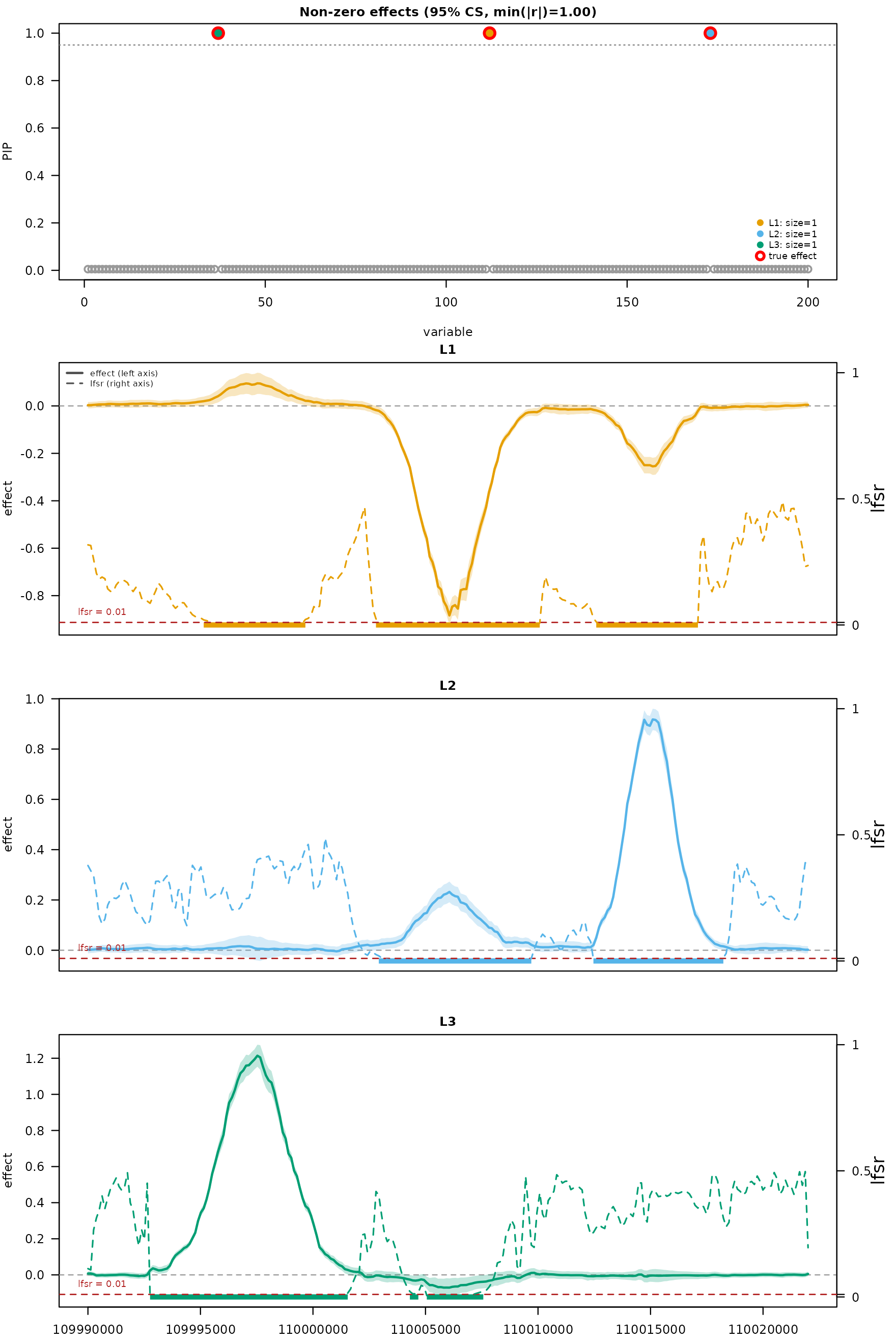
The three CS effect curves capture three separate gene-body regions, mirroring the multi-CS structure in published GTEx fSuSiE figures.
Genome-browser overlay (Gviz)
For a publication-grade figure with chromosome ideogram, genome axis,
fitted effect track, observed allele-stratified coverage, and read-count
tracks, mfsusieR ships a worked example using
Gviz. The Bioconductor packages it depends on
(Gviz, GenomicRanges, IRanges)
are listed as Suggests only.
suppressPackageStartupMessages({
  library(Gviz); library(GenomicRanges); library(IRanges)
})

n_cs   <- length(fit_s$sets$cs)
chrom  <- gtex_example$chrom
pos    <- gtex_example$pos
gr     <- GRanges(chrom, IRanges(pos, pos + 1L))

# Default smoother on this fit is TI; its result lives at
# `fit_s$smoothed$TI`.
smooth_payload <- fit_s$smoothed$TI
cs_palette <- c("#1f78b4", "#33a02c", "#e31a1c", "#ff7f00",
                "#6a3d9a", "#b15928")[seq_len(n_cs)]

# Build one effect track per CS: solid mean line + two dashed
# credible-band lines, layered via OverlayTrack.
effect_tracks <- lapply(seq_len(n_cs), function(cs) {
  band   <- smooth_payload$credible_bands[[1L]][[cs]]
  effect <- smooth_payload$effect_curves[[1L]][[cs]]
  ylim_e <- range(c(effect, band)) * c(1.1, 1.1)
  e_main <- DataTrack(range = gr, data = effect, type = "l", lwd = 2,
                      col = cs_palette[cs],
                      name = sprintf("CS %d", cs),
                      ylim = ylim_e,
                      background.title = "white",
                      col.axis = "black", col.title = "black",
                      fontface.title = 1)
  e_lo   <- DataTrack(range = gr, data = band[, 1L], type = "l",
                      lty = 2, col = cs_palette[cs], ylim = ylim_e)
  e_hi   <- DataTrack(range = gr, data = band[, 2L], type = "l",
                      lty = 2, col = cs_palette[cs], ylim = ylim_e)
  OverlayTrack(trackList = list(e_main, e_lo, e_hi),
               background.title = "white")
})

# Use CS 1 lead variant for the allele-stratified coverage panel
# (one panel; coloring by all leads gets cluttered).
markers_1 <- fit_s$sets$cs[[1L]]
lead_1    <- markers_1[which.max(fit_s$pip[markers_1])]
x_lead_1  <- gtex_example$X[, lead_1]
g0 <- which(x_lead_1 < 0)
g1 <- which(x_lead_1 >= 0)
mu0 <- colMeans(gtex_example$Y[g0, , drop = FALSE])
mu1 <- colMeans(gtex_example$Y[g1, , drop = FALSE])

ylim_c <- range(c(mu0, mu1))
c_ref  <- DataTrack(range = gr, data = mu0, type = "p", pch = 16,
                    cex = 0.5, col = "navy",
                    name = "Avg log1p (CS 1 lead split)",
                    ylim = ylim_c,
                    background.title = "white", col.axis = "black",
                    col.title = "black", fontface.title = 1)
c_alt  <- DataTrack(range = gr, data = mu1, type = "p", pch = 16,
                    cex = 0.5, col = "turquoise", ylim = ylim_c)
count_track <- OverlayTrack(trackList = list(c_ref, c_alt),
                            background.title = "white")

axis_track <- GenomeAxisTrack(col = "black", fontcolor = "black",
                              col.title = "black",
                              background.title = "white")

gene_track <- GeneRegionTrack(gtex_example$gene_track,
                              chromosome = chrom,
                              name = "", showId = TRUE,
                              geneSymbol = TRUE,
                              col = "salmon", fill = "salmon",
                              background.title = "white",
                              col.axis = "black", col.title = "black")

# Each effect track gets equal vertical real estate; coverage
# track gets 1.5x; gene track gets 2x.
track_sizes <- c(1, rep(2, n_cs), 2.5, 2)
cs_leads <- vapply(fit_s$sets$cs, function(idx)
  idx[which.max(fit_s$pip[idx])], integer(1L))
plotTracks(c(list(axis_track), effect_tracks,
             list(count_track, gene_track)),
           from  = gtex_example$locus[1L],
           to    = gtex_example$locus[2L],
           sizes = track_sizes,
           main  = sprintf("%s cis-eQTL: %d credible sets at SNPs %s",
                           gtex_example$gene, n_cs,
                           paste(cs_leads, collapse = ", ")),
           cex.main = 1.0)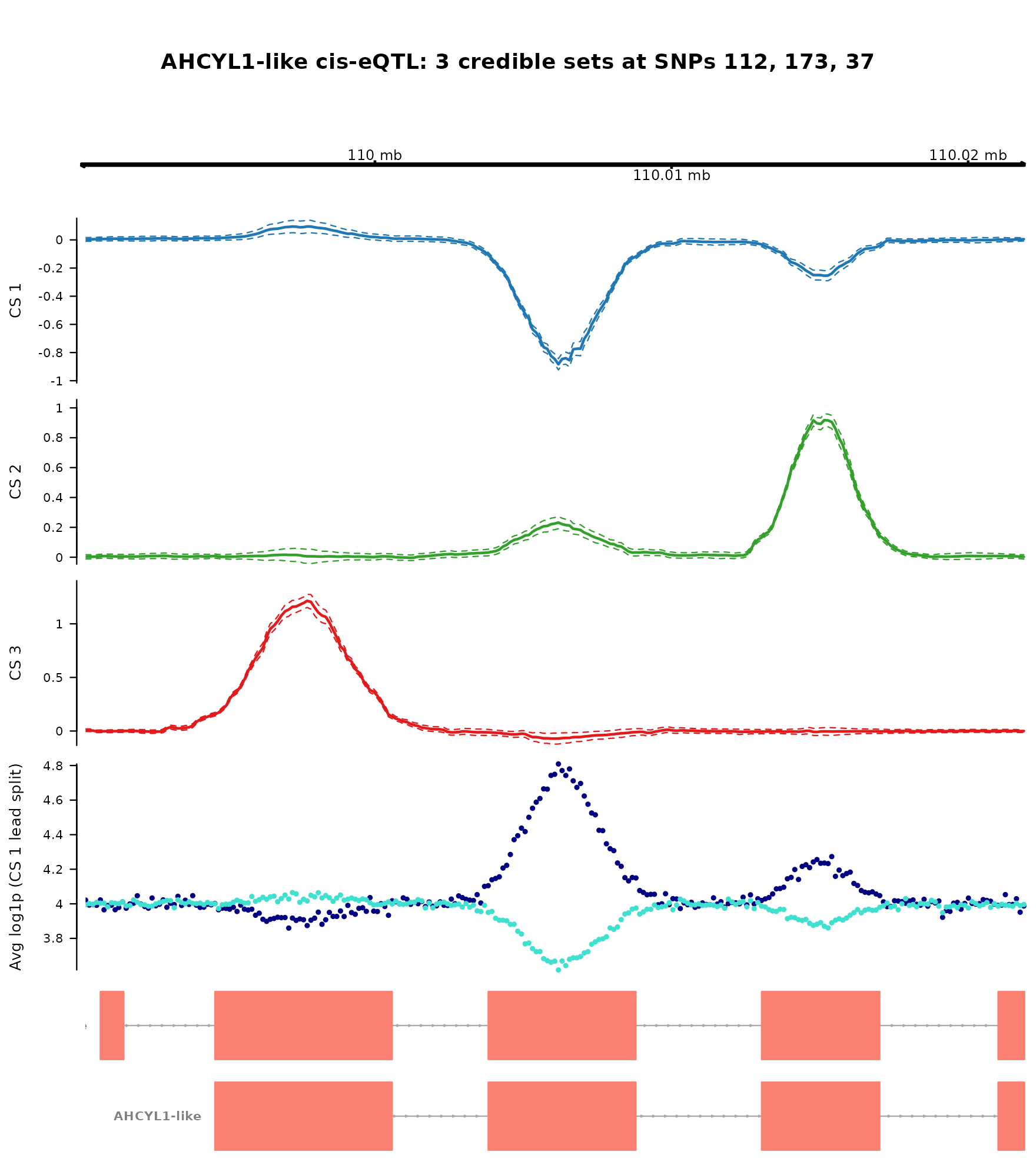
The Gviz figure layout consists of top axis with positions in the
gene-body window, the fSuSiE effect curve with dashed credible band, the
observed allele-stratified coverage difference at each gene-body
position, and the per-position log1p counts split by genotype class.
Adding an IdeogramTrack from a real chromosome and a
GeneRegionTrack from a TxDb package (e.g.
TxDb.Hsapiens.UCSC.hg38.knownGene) extends this to a full
ideogram + transcript layout; the worked-example scripts in
system.file("scripts/gtex_case_study", package = "mfsusieR")
show the wiring on a real (chrom, gene) pair when the
underlying RNA-seq data is available locally.
Why functional fine-mapping helps here
The fine-mapping signal is spread across many positions of the gene.
A scalar SuSiE fit on rowSums(Y) (total expression) mixes
every per-position effect into one number and loses the per-region
structure. The functional model preserves it:
library(susieR)
fit_scalar <- susie(gtex_example$X, rowSums(gtex_example$Y),
                    L = 15, verbose = FALSE)
fit_scalar$sets$cs
#> $L1
#> [1] 37
#>
#> $L2
#> [1] 112
#>
#> $L3
#> [1] 173
fit_scalar$pip[gtex_example$causal_snps]
#> [1] 1 1 1
Per-position effects are not recoverable from the scalar fit; they
are the natural output of fsusie().
Session info
This is the version of R and the packages that were used to generate these results.
sessionInfo()
#> R version 4.4.3 (2025-02-28)
#> Platform: x86_64-conda-linux-gnu
#> Running under: Ubuntu 24.04.4 LTS
#>
#> Matrix products: default
#> BLAS/LAPACK: /home/runner/work/mfsusieR/mfsusieR/.pixi/envs/r44/lib/libopenblasp-r0.3.32.so;  LAPACK version 3.12.0
#>
#> locale:
#>  [1] LC_CTYPE=C.UTF-8       LC_NUMERIC=C           LC_TIME=C.UTF-8
#>  [4] LC_COLLATE=C.UTF-8     LC_MONETARY=C.UTF-8    LC_MESSAGES=C.UTF-8
#>  [7] LC_PAPER=C.UTF-8       LC_NAME=C              LC_ADDRESS=C
#> [10] LC_TELEPHONE=C         LC_MEASUREMENT=C.UTF-8 LC_IDENTIFICATION=C
#>
#> time zone: Etc/UTC
#> tzcode source: system (glibc)
#>
#> attached base packages:
#> [1] grid      stats4    stats     graphics  grDevices utils     datasets
#> [8] methods   base
#>
#> other attached packages:
#> [1] susieR_0.16.1        Gviz_1.50.0          GenomicRanges_1.58.0
#> [4] GenomeInfoDb_1.42.0  IRanges_2.40.0       S4Vectors_0.44.0
#> [7] BiocGenerics_0.52.0  mfsusieR_0.0.2
#>
#> loaded via a namespace (and not attached):
#>   [1] RColorBrewer_1.1-3          rstudioapi_0.18.0
#>   [3] jsonlite_2.0.0              magrittr_2.0.5
#>   [5] GenomicFeatures_1.58.0      farver_2.1.2
#>   [7] rmarkdown_2.31              fs_2.1.0
#>   [9] BiocIO_1.16.0               zlibbioc_1.52.0
#>  [11] ragg_1.5.2                  vctrs_0.7.3
#>  [13] memoise_2.0.1               Rsamtools_2.22.0
#>  [15] RCurl_1.98-1.18             SQUAREM_2026.1
#>  [17] base64enc_0.1-6             mixsqp_0.3-54
#>  [19] htmltools_0.5.9             S4Arrays_1.6.0
#>  [21] progress_1.2.3              curl_7.1.0
#>  [23] truncnorm_1.0-9             SparseArray_1.6.0
#>  [25] Formula_1.2-5               sass_0.4.10
#>  [27] bslib_0.10.0                htmlwidgets_1.6.4
#>  [29] desc_1.4.3                  plyr_1.8.9
#>  [31] httr2_1.2.2                 cachem_1.1.0
#>  [33] GenomicAlignments_1.42.0    lifecycle_1.0.5
#>  [35] pkgconfig_2.0.3             Matrix_1.7-5
#>  [37] R6_2.6.1                    fastmap_1.2.0
#>  [39] GenomeInfoDbData_1.2.13     MatrixGenerics_1.18.0
#>  [41] digest_0.6.39               reshape_0.8.10
#>  [43] colorspace_2.1-2            AnnotationDbi_1.68.0
#>  [45] irlba_2.3.7                 textshaping_1.0.5
#>  [47] Hmisc_5.2-5                 RSQLite_2.4.6
#>  [49] invgamma_1.2                filelock_1.0.3
#>  [51] deconvolveR_1.2-1           httr_1.4.8
#>  [53] abind_1.4-8                 compiler_4.4.3
#>  [55] horseshoe_0.2.0             bit64_4.8.0
#>  [57] htmlTable_2.5.0             S7_0.2.2
#>  [59] backports_1.5.1             BiocParallel_1.40.0
#>  [61] DBI_1.3.0                   biomaRt_2.62.0
#>  [63] MASS_7.3-65                 rappdirs_0.3.4
#>  [65] DelayedArray_0.32.0         rjson_0.2.23
#>  [67] tools_4.4.3                 trust_0.1-9
#>  [69] foreign_0.8-91              otel_0.2.0
#>  [71] ebnm_1.0-55                 nnet_7.3-20
#>  [73] glue_1.8.1                  restfulr_0.0.16
#>  [75] checkmate_2.3.3             cluster_2.1.8.2
#>  [77] generics_0.1.4              gtable_0.3.6
#>  [79] BSgenome_1.74.0             ensembldb_2.30.0
#>  [81] data.table_1.17.8           hms_1.1.4
#>  [83] xml2_1.5.2                  XVector_0.46.0
#>  [85] pillar_1.11.1               stringr_1.6.0
#>  [87] splines_4.4.3               dplyr_1.2.1
#>  [89] BiocFileCache_2.14.0        lattice_0.22-9
#>  [91] rtracklayer_1.66.0          bit_4.6.0
#>  [93] deldir_2.0-4                biovizBase_1.54.0
#>  [95] tidyselect_1.2.1            Biostrings_2.74.0
#>  [97] knitr_1.51                  gridExtra_2.3
#>  [99] ProtGenerics_1.38.0         SummarizedExperiment_1.36.0
#> [101] xfun_0.57                   Biobase_2.66.0
#> [103] matrixStats_1.5.0           LaplacesDemon_16.1.8
#> [105] stringi_1.8.7               UCSC.utils_1.2.0
#> [107] lazyeval_0.2.3              yaml_2.3.12
#> [109] evaluate_1.0.5              codetools_0.2-20
#> [111] interp_1.1-6                tibble_3.3.1
#> [113] cli_3.6.6                   RcppParallel_5.1.11-2
#> [115] rpart_4.1.27                systemfonts_1.3.2
#> [117] jquerylib_0.1.4             dichromat_2.0-0.1
#> [119] Rcpp_1.1.1-1.1              zigg_0.0.2
#> [121] dbplyr_2.5.2                png_0.1-9
#> [123] Rfast_2.1.5.2               XML_3.99-0.23
#> [125] parallel_4.4.3              pkgdown_2.2.0
#> [127] ggplot2_4.0.3               blob_1.3.0
#> [129] prettyunits_1.2.0           latticeExtra_0.6-31
#> [131] jpeg_0.1-11                 wavethresh_4.7.3
#> [133] AnnotationFilter_1.30.0     bitops_1.0-9
#> [135] VariantAnnotation_1.52.0    scales_1.4.0
#> [137] crayon_1.5.3                rlang_1.2.0
#> [139] ashr_2.2-63                 KEGGREST_1.46.0