Adjusting for covariates in functional fine-mapping

This vignette adjusts a functional response Y for covariate effects before fine-mapping. Observed covariates that affect the trait at every position (age, sex, batch, principal components of a global expression matrix) inflate the residual variance and attenuate the genetic signal if left in. The right tool for removing such effects on a functional response is a wavelet- domain empirical-Bayes regression that accommodates smooth position-dependent covariate effects. mfsusieR exposes this through mf_adjust_for_covariates().

Setup

library(mfsusieR)
library(susieR)
library(wavethresh)
set.seed(2L)

Generating the data

We simulate functional responses with two ingredients:

Genetic signal — two causal SNPs (positions 25 and 75 in the genotype matrix) with smooth random per-position effects f1, f2.
Covariate signal — three covariates (independent of genotype) acting through smooth random per-position coefficient curves f1_cov, f2_cov, f3_cov.

All effect curves are drawn from mf_simu_ibss_per_level(7)$sim_func, which samples from the IBSS wavelet prior (the same prior class fSuSiE infers).

rsnr    <- 1
pos1    <- 25L
pos2    <- 75L
lev_res <- 7L
T_m     <- 2L^lev_res

f1     <- mf_simu_ibss_per_level(lev_res)$sim_func
f2     <- mf_simu_ibss_per_level(lev_res)$sim_func
f1_cov <- mf_simu_ibss_per_level(lev_res)$sim_func
f2_cov <- mf_simu_ibss_per_level(lev_res)$sim_func
f3_cov <- mf_simu_ibss_per_level(lev_res)$sim_func

plot(f1, type = "l", col = "royalblue", lwd = 2,
     xlab = "position", ylab = "effect")
abline(h = 0, lty = 3, col = "grey50")
lines(f2, type = "l", col = "limegreen", lwd = 2)
legend("topright", legend = c("f1 (SNP 25)", "f2 (SNP 75)"),
       col = c("royalblue", "limegreen"), lwd = 2, bty = "n")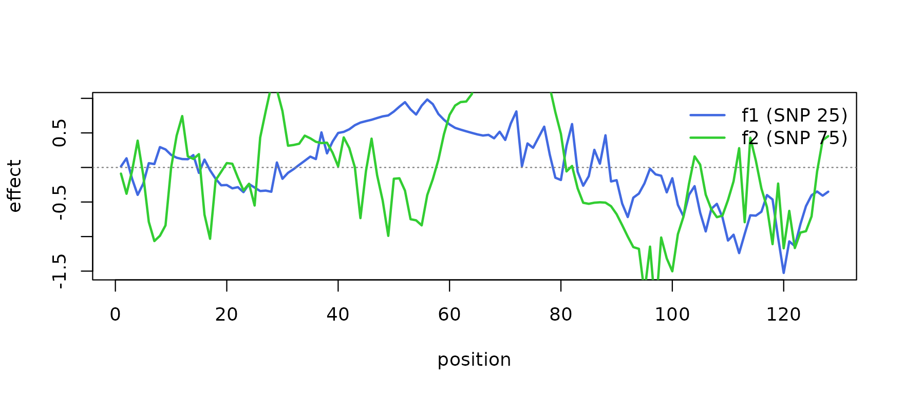

The observed data is a mixture of covariate-driven confounding and genotype signal. genetic_signal is the part we want to recover; covariate_signal is the part we want to remove.

data(N3finemapping)
Geno <- N3finemapping$X[, seq_len(100)]
n    <- nrow(Geno)

# Three covariates, sd = 2; independent of Geno.
Cov <- matrix(rnorm(3L * n, sd = 2), ncol = 3L)

genetic_signal   <- matrix(0, n, T_m)
covariate_signal <- matrix(0, n, T_m)
for (i in seq_len(n)) {
  noise_i <- rnorm(T_m, sd = (1 / rsnr) * var(f1))
  genetic_signal[i, ] <-
    Geno[i, pos1] * f1 + Geno[i, pos2] * f2 + noise_i
  covariate_signal[i, ] <-
    Cov[i, 1L] * f1_cov + Cov[i, 2L] * f2_cov + Cov[i, 3L] * f3_cov
}
Y <- covariate_signal + genetic_signal

The covariate signal dominates the per-position scale of Y, so without adjustment fSuSiE’s recovered effect curves are biased toward the covariate-induced confounding rather than the true genetic effect.

Account for covariates

mf_adjust_for_covariates(Y, Cov, method = "wavelet_eb") fits a wavelet-domain empirical-Bayes regression of Y on the covariates Cov and returns the residualised response Y_adjusted = Y - Cov %*% fitted_func along with the fitted covariate effect curves.

adj <- mf_adjust_for_covariates(Y, Cov)
str(adj, max.level = 1L)
#> List of 7
#>  $ Y_adjusted : num [1:574, 1:128] 0.125 0.762 -0.284 0.222 -0.473 ...
#>  $ X_adjusted : NULL
#>  $ fitted_func: num [1:3, 1:128] 1.354 -0.268 -0.51 1.414 -0.41 ...
#>  $ sigma2     : num 0.424
#>  $ niter      : int 5
#>  $ converged  : logi TRUE
#>  $ method     : chr "wavelet_eb"

The first row of adj$fitted_func is the recovered effect of the first covariate on the response curve; overlay it on the truth f1_cov:

plot(adj$fitted_func[1L, ], type = "l", col = "blue",
     lty = 2, lwd = 2,
     xlab = "position", ylab = "covariate effect",
     main = "Covariate 1: estimated vs true")
lines(f1_cov, lwd = 1.5)
legend("topright", lwd = c(1.5, 2), lty = c(1, 2),
       legend = c("true f1_cov", "estimated"), bty = "n")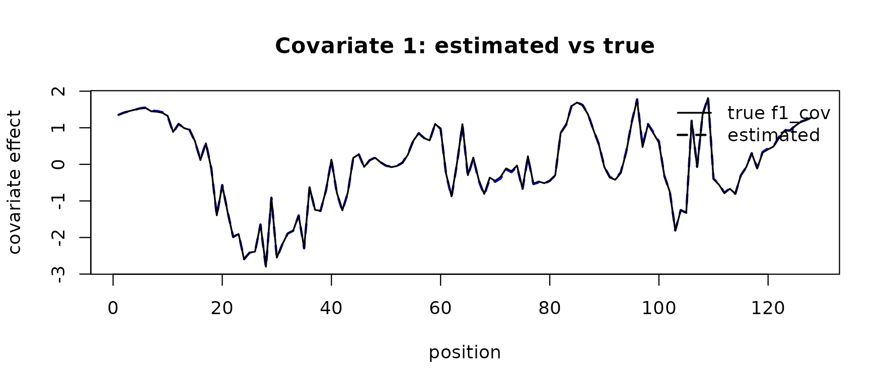

adj$Y_adjusted is the residualised response on the original position grid, ready to feed into fsusie().

Recovering the genetic signal

A two-panel scatter shows that the adjusted response tracks the genetic-only signal far more tightly than the raw response:

par(mfrow = c(1L, 2L))
plot(Y, genetic_signal, pch = 19L, cex = 0.4,
     xlab = "Observed Y", ylab = "Genetic signal",
     main = "Before adjustment")
abline(0, 1, lty = 3, col = "grey50")
plot(adj$Y_adjusted, genetic_signal, pch = 19L, cex = 0.4,
     xlab = "Y adjusted", ylab = "Genetic signal",
     main = "After adjustment")
abline(0, 1, lty = 3, col = "grey50")

par(mfrow = c(1L, 1L))

Fine-mapping the adjusted response

fit_adj <- fsusie(adj$Y_adjusted, Geno)
fit_adj$sets$cs
#> $L1
#> [1] 75 83
#> 
#> $L2
#> [1] 25
fit_adj$pip[c(pos1, pos2)]
#> [1] 1.0000000 0.5001951

plot_dims <- mfsusie_plot_dimensions(fit_adj)

mfsusie_plot(fit_adj, effect_variables = c(pos1, pos2))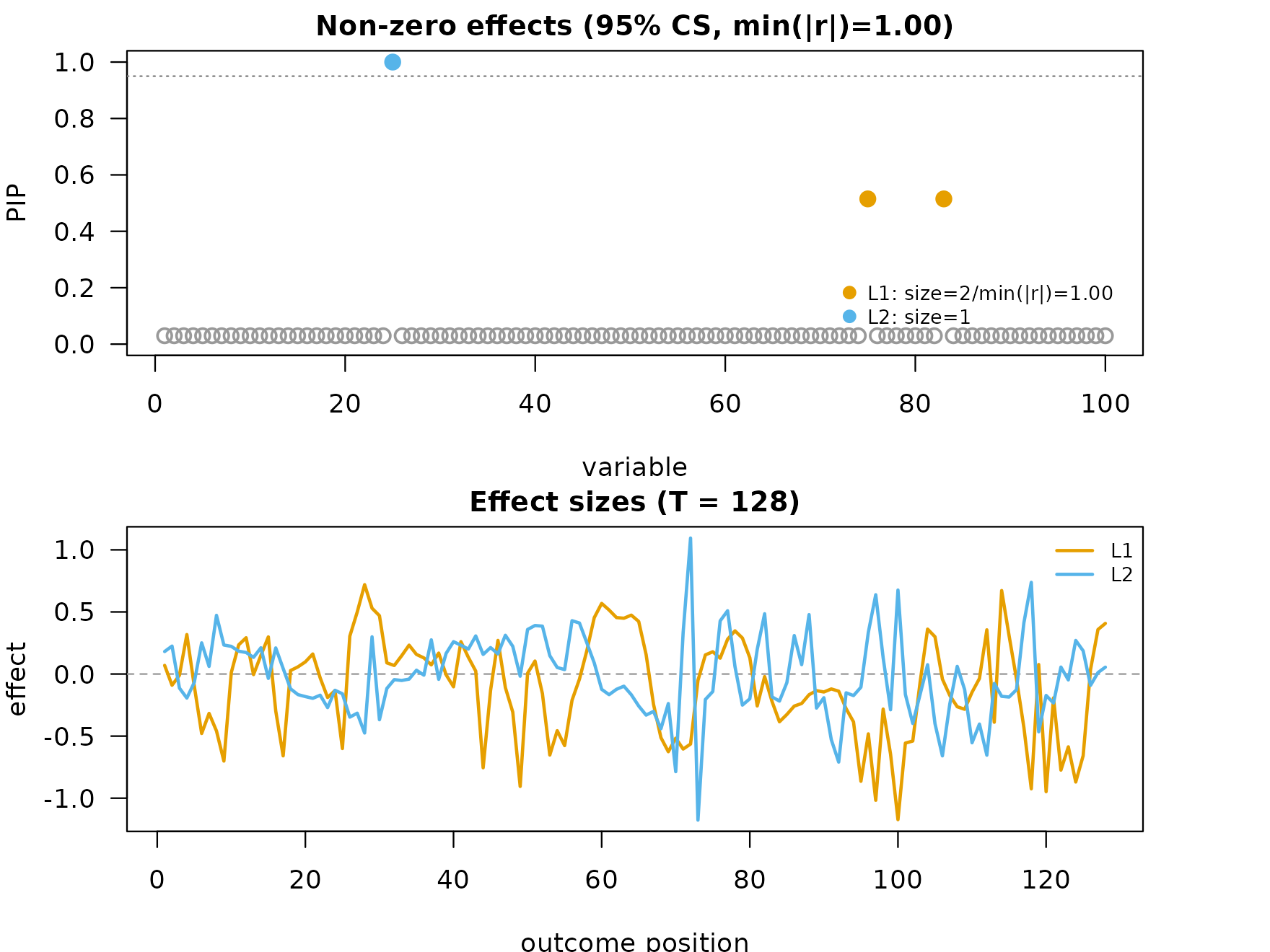

Comparison with no adjustment

For contrast, fit fsusie() directly on Y without adjustment:

fit_unadj <- fsusie(Y, Geno)
fit_unadj$sets$cs
#> $L1
#> [1] 75 83
#> 
#> $L3
#> [1] 48
#> 
#> $L4
#> [1] 94
#> 
#> $L5
#> [1] 97
#> 
#> $L6
#> [1] 57
#> 
#> $L7
#> [1] 60
#> 
#> $L2
#> [1] 24 26
fit_unadj$pip[c(pos1, pos2)]
#> [1] 0.0001472286 0.5000000000

fsusie() returns raw inverse-DWT effect curves via coef(); position-space smoothing with a 95% credible band is an opt-in post-processing step. Run mf_post_smooth(fit, method = "TI") on each fit to get translation-invariant cycle-spun curves, then read them back via coef(fit_s, smooth_method = "TI"). Match each fitted CS to its causal SNP by lead-PIP and overlay the smoothed recovered curve from each fit against the ground-truth f1 and f2.

fit_adj_s   <- mf_post_smooth(fit_adj,   method = "TI")
fit_unadj_s <- mf_post_smooth(fit_unadj, method = "TI")
cf_adj   <- coef(fit_adj_s,   smooth_method = "TI")[[1L]]
cf_unadj <- coef(fit_unadj_s, smooth_method = "TI")[[1L]]

match_cs <- function(fit, target_snp) {
  if (length(fit$sets$cs) == 0L) return(NA_integer_)
  leads <- vapply(fit$sets$cs, function(idx) {
    idx[which.max(fit$pip[idx])]
  }, integer(1L))
  hit <- which(leads == target_snp)
  if (length(hit) == 0L) NA_integer_ else hit[1L]
}

plot_effect <- function(snp, truth, col, label) {
  l_adj   <- match_cs(fit_adj,   snp)
  l_unadj <- match_cs(fit_unadj, snp)
  rec_adj   <- if (!is.na(l_adj))   cf_adj[l_adj, ]     else NULL
  rec_unadj <- if (!is.na(l_unadj)) cf_unadj[l_unadj, ] else NULL
  yrng <- range(c(truth, rec_adj, rec_unadj), na.rm = TRUE)
  plot(truth, pch = 20L, col = "grey30", cex = 0.7,
       xlab = "position", ylab = "effect", ylim = yrng,
       main = paste("Estimated effect:", label))
  abline(h = 0, lty = 3, col = "grey50")
  if (!is.null(rec_adj))   lines(rec_adj,   col = col, lwd = 1.8)
  if (!is.null(rec_unadj)) lines(rec_unadj, col = col, lwd = 1.5, lty = 2)
  legend("topright",
         legend = c("truth", "fSuSiE adjusted", "fSuSiE unadjusted"),
         col    = c("grey30", col, col),
         lty    = c(NA, 1, 2), lwd = c(NA, 1.8, 1.5),
         pch    = c(20, NA, NA), bty = "n", cex = 0.85)
}

Estimated effect 1 (true causal at SNP 25):

plot_effect(pos1, f1, "blue", "f1 (SNP 25)")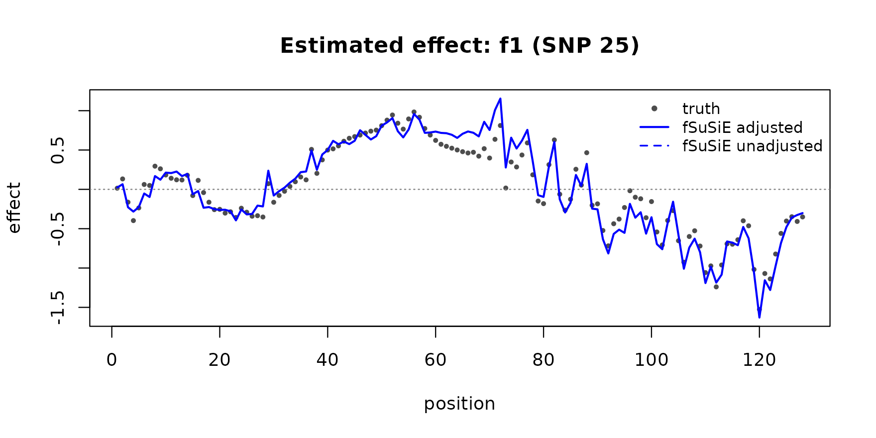

Estimated effect 2 (true causal at SNP 75):

plot_effect(pos2, f2, "darkgreen", "f2 (SNP 75)")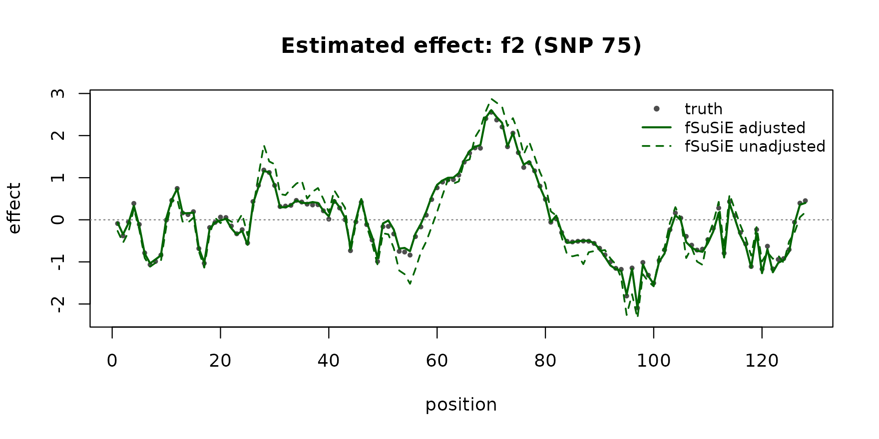

The TI-smoothed adjusted-fit curves track the truth on both signals at near-perfect correlation. The unadjusted fit is biased toward the covariate-induced confounding and the recovered curves drift away from the truth.

Scalar traits: OLS adjustment with the FWL correction

When the response is a scalar (T = 1) or smoothness across positions is irrelevant, the closed-form OLS residualization is the right tool. Pass method = "ols" to use it. When the covariates are correlated with genotype, also pass X so the function returns the Frisch-Waugh-Lovell-corrected X_adjusted:

# Scalar response derived from the same covariate-confounded
# data: take the per-individual mean of Y as the scalar trait
# and wrap it as a single-column matrix.
Y_scalar <- matrix(rowMeans(Y), ncol = 1L)

adj_ols <- mf_adjust_for_covariates(Y_scalar, Cov, X = Geno,
                                    method = "ols")
str(adj_ols, max.level = 1L)
#> List of 4
#>  $ Y_adjusted : num [1:574, 1] -0.00905 0.03383 -0.04059 0.03828 0.00103 ...
#>  $ X_adjusted : num [1:574, 1:100] -0.0171 -0.0109 -0.0104 -0.0107 -0.0458 ...
#>  $ fitted_func: num [1:3, 1] -3.88e-05 -4.15e-04 -5.67e-04
#>  $ method     : chr "ols"

adj_ols returns:

Y_adjusted: the scalar response after projecting out the covariate column space.
X_adjusted: the genotype matrix after the same projection (the FWL correction). When Cov is correlated with Geno, using X_adjusted instead of the original Geno removes the bias in the downstream fit.

A scalar susie() fit on the OLS-adjusted data:

fit_scalar <- susieR::susie(adj_ols$X_adjusted,
                            as.numeric(adj_ols$Y_adjusted),
                            L = 5L, verbose = FALSE)
fit_scalar$sets$cs
#> NULL
fit_scalar$pip[c(pos1, pos2)]
#> [1] 0 0

For T > 1 use method = "wavelet_eb" (the default demonstrated above). Use method = "ols" for scalar traits or when smooth covariate effects across positions are not expected.

Next steps

For colocalization across two functional fits, see the colocalization vignette. For post-fit smoothing of effect curves, see the post-processing vignette.

Session info

This is the version of R and the packages that were used to generate these results.

sessionInfo()
#> R version 4.4.3 (2025-02-28)
#> Platform: x86_64-conda-linux-gnu
#> Running under: Ubuntu 24.04.4 LTS
#> 
#> Matrix products: default
#> BLAS/LAPACK: /home/runner/work/mfsusieR/mfsusieR/.pixi/envs/r44/lib/libopenblasp-r0.3.32.so;  LAPACK version 3.12.0
#> 
#> locale:
#>  [1] LC_CTYPE=C.UTF-8       LC_NUMERIC=C           LC_TIME=C.UTF-8       
#>  [4] LC_COLLATE=C.UTF-8     LC_MONETARY=C.UTF-8    LC_MESSAGES=C.UTF-8   
#>  [7] LC_PAPER=C.UTF-8       LC_NAME=C              LC_ADDRESS=C          
#> [10] LC_TELEPHONE=C         LC_MEASUREMENT=C.UTF-8 LC_IDENTIFICATION=C   
#> 
#> time zone: Etc/UTC
#> tzcode source: system (glibc)
#> 
#> attached base packages:
#> [1] stats     graphics  grDevices utils     datasets  methods   base     
#> 
#> other attached packages:
#> [1] wavethresh_4.7.3 MASS_7.3-65      susieR_0.16.1    mfsusieR_0.0.2  
#> 
#> loaded via a namespace (and not attached):
#>  [1] sass_0.4.10           generics_0.1.4        ashr_2.2-63          
#>  [4] lattice_0.22-9        digest_0.6.39         magrittr_2.0.5       
#>  [7] evaluate_1.0.5        grid_4.4.3            RColorBrewer_1.1-3   
#> [10] fastmap_1.2.0         plyr_1.8.9            jsonlite_2.0.0       
#> [13] Matrix_1.7-5          reshape_0.8.10        mixsqp_0.3-54        
#> [16] scales_1.4.0          truncnorm_1.0-9       invgamma_1.2         
#> [19] textshaping_1.0.5     jquerylib_0.1.4       cli_3.6.6            
#> [22] crayon_1.5.3          zigg_0.0.2            rlang_1.2.0          
#> [25] deconvolveR_1.2-1     LaplacesDemon_16.1.8  splines_4.4.3        
#> [28] cachem_1.1.0          yaml_2.3.12           otel_0.2.0           
#> [31] ebnm_1.0-55           tools_4.4.3           SQUAREM_2026.1       
#> [34] parallel_4.4.3        dplyr_1.2.1           ggplot2_4.0.3        
#> [37] Rfast_2.1.5.2         vctrs_0.7.3           R6_2.6.1             
#> [40] matrixStats_1.5.0     lifecycle_1.0.5       fs_2.1.0             
#> [43] htmlwidgets_1.6.4     trust_0.1-9           ragg_1.5.2           
#> [46] irlba_2.3.7           pkgconfig_2.0.3       desc_1.4.3           
#> [49] RcppParallel_5.1.11-2 pkgdown_2.2.0         bslib_0.10.0         
#> [52] pillar_1.11.1         gtable_0.3.6          glue_1.8.1           
#> [55] Rcpp_1.1.1-1.1        systemfonts_1.3.2     xfun_0.57            
#> [58] tibble_3.3.1          tidyselect_1.2.1      dichromat_2.0-0.1    
#> [61] knitr_1.51            farver_2.1.2          htmltools_0.5.9      
#> [64] rmarkdown_2.31        compiler_4.4.3        S7_0.2.2             
#> [67] horseshoe_0.2.0

William Denault