Summary Statistics Data Colocalization
Source:vignettes/Summary_Statistics_Colocalization.Rmd
Summary_Statistics_Colocalization.RmdThis vignette demonstrates how to perform multi-trait colocalization
analysis using summary statistics data, specifically focusing on the
Sumstat_5traits dataset included in the package.
1. The Sumstat_5traits Dataset
The Sumstat_5traits dataset contains 5 simulated summary
statistics, where it is directly derived from the
Ind_5traits dataset using marginal association. The dataset
is specifically designed to evaluate and demonstrate the capabilities of
ColocBoost in multi-trait colocalization analysis with summary
association data.
-
sumstat: A list of data.frames of summary statistics for different traits. -
true_effect_variants: True effect variants indices for each trait. - Note that
LDcould be calculated from theXdata in theInd_5traitsdataset, but it is not included in theSumstat_5traitsdataset.
Causal variant structure
The dataset features two causal variants with indices 194 and 589.
- Causal variant 194 is associated with traits 1, 2, 3, and 4.
- Causal variant 589 is associated with traits 2, 3, and 5.
This structure creates a realistic scenario in which multiple traits are influenced by different but overlapping sets of genetic variants.
# Loading the Dataset
data("Sumstat_5traits")
names(Sumstat_5traits)
#> [1] "sumstat"              "true_effect_variants"
Sumstat_5traits$true_effect_variants
#> $Outcome_1
#> [1] 194
#>
#> $Outcome_2
#> [1] 194 589
#>
#> $Outcome_3
#> [1] 194 589
#>
#> $Outcome_4
#> [1] 194
#>
#> $Outcome_5
#> [1] 589
Due to the file size limitation of CRAN release, this is a subset of simulated data. See full dataset in colocboost paper repo.
Important data format for summary data
sumstat must include the following columns:
-
zor (beta,sebeta): either z-score or (effect size and standard error) -
n: sample size for the summary statistics. Highly recommended: Providing the sample size, or even a rough estimate ofn, is highly recommended. Withoutn, the implicit assumption isnis large (Inf) and the effect sizes are small (close to zero). -
variant: required ifsumstatfor different outcomes do not have the same number of variables (multiplesumstatand multipleLD).
2. Multiple summary statistics data with shared LD reference
The preferred format for colocalization analysis in ColocBoost using summary statistics data is where one LD matrix is provided for all traits, and the summary statistics are organized in a list. The Basic format is
-
sumstatis organized as a list of data.frames for all traits -
LDis a matrix of linkage disequilibrium (LD) information for all variants across all traits.
This function requires specifying summary statistics
sumstat and LD matrix LD from the dataset:
# Extract genotype (X) and calculate LD matrix
data("Ind_5traits")
LD <- get_cormat(Ind_5traits$X[[1]])

# Run colocboost
res <- colocboost(sumstat = Sumstat_5traits$sumstat, LD = LD)
#> Validating input data.
#> Starting gradient boosting algorithm.
#> Gradient boosting for outcome 4 converged after 40 iterations!
#> Gradient boosting for outcome 5 converged after 59 iterations!
#> Gradient boosting for outcome 1 converged after 61 iterations!
#> Gradient boosting for outcome 3 converged after 91 iterations!
#> Gradient boosting for outcome 2 converged after 94 iterations!
#> Performing inference on colocalization events.
#> Extracting colocalization results with pvalue_cutoff = 0.001, cos_npc_cutoff = 0.2, and npc_outcome_cutoff = 0.2.
#> Keep only CoS with cos_npc >= 0.2. For each CoS, keep the outcomes configurations that pvalue of variants for the outcome < 0.001 and npc_outcome >0.2.

# Identified CoS
res$cos_details$cos$cos_index
#> $`cos1:y1_y2_y3_y4`
#> [1] 186 194 168 205
#>
#> $`cos2:y2_y3_y5`
#> [1] 589 593

# Plotting the results
colocboost_plot(res)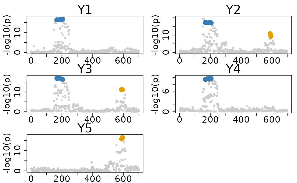
Alternatively, you can provide the reference panel genotype matrix
directly through X_ref, which avoids storing the full LD
matrix:
# Use reference genotype directly instead of precomputing LD
X_ref <- Ind_5traits$X[[1]]

# Run colocboost
res <- colocboost(sumstat = Sumstat_5traits$sumstat, X_ref = X_ref)
#> Validating input data.
#> N_ref >= P: precomputing LD from X_ref.
#> Starting gradient boosting algorithm.
#> Gradient boosting for outcome 4 converged after 40 iterations!
#> Gradient boosting for outcome 5 converged after 59 iterations!
#> Gradient boosting for outcome 1 converged after 61 iterations!
#> Gradient boosting for outcome 3 converged after 91 iterations!
#> Gradient boosting for outcome 2 converged after 94 iterations!
#> Performing inference on colocalization events.
#> Extracting colocalization results with pvalue_cutoff = 0.001, cos_npc_cutoff = 0.2, and npc_outcome_cutoff = 0.2.
#> Keep only CoS with cos_npc >= 0.2. For each CoS, keep the outcomes configurations that pvalue of variants for the outcome < 0.001 and npc_outcome >0.2.

# Identified CoS
res$cos_details$cos$cos_index
#> $`cos1:y1_y2_y3_y4`
#> [1] 186 194 168 205
#>
#> $`cos2:y2_y3_y5`
#> [1] 589 593
Results Interpretation
For comprehensive tutorials on result interpretation and advanced visualization techniques, please visit our tutorials portal at Visualization of ColocBoost Results and Interpret ColocBoost Output.
3. Other summary statistics and LD input combinations
3.1. Matched LD with multiple sumstat (Trait-specific LD)
When studying multiple traits with their own trait-specific LD matrices, you could provide a list of LD matrices matched with a list of summary statistics.
-
Basic format:
sumstatandLDare organized as lists, matched by trait index,-
(sumstat[1], LD[1])contains information for trait 1, -
(sumstat[2], LD[2])contains information for trait 2, - And so on for each trait under analysis.
-
-
Cross-trait flexibility:
- There is no requirement for the same variants across different traits. This allows for the analysis of traits with available variants.
- This is particularly useful when you have a large dataset with many traits and want to focus on specific variants and trait-specific LD.
# Duplicate LD with matched summary statistics
LD_multiple <- lapply(1:length(Sumstat_5traits$sumstat), function(i) LD )

# Run colocboost
res <- colocboost(sumstat = Sumstat_5traits$sumstat, LD = LD_multiple)
#> Validating input data.
#> Starting gradient boosting algorithm.
#> Gradient boosting for outcome 4 converged after 40 iterations!
#> Gradient boosting for outcome 5 converged after 59 iterations!
#> Gradient boosting for outcome 1 converged after 61 iterations!
#> Gradient boosting for outcome 3 converged after 91 iterations!
#> Gradient boosting for outcome 2 converged after 94 iterations!
#> Performing inference on colocalization events.
#> Extracting colocalization results with pvalue_cutoff = 0.001, cos_npc_cutoff = 0.2, and npc_outcome_cutoff = 0.2.
#> Keep only CoS with cos_npc >= 0.2. For each CoS, keep the outcomes configurations that pvalue of variants for the outcome < 0.001 and npc_outcome >0.2.

# Identified CoS
res$cos_details$cos$cos_index
#> $`cos1:y1_y2_y3_y4`
#> [1] 186 194 168 205
#>
#> $`cos2:y2_y3_y5`
#> [1] 589 593
3.2. LD matrix is a superset of variants across different summary statistics
When the LD matrix includes a superset of variants across different summary statistics, with Input Format:
-
sumstatis a list of data.frames for all traits -
LDis a matrix of linkage disequilibrium (LD) information for all variants across all traits. - The LD matrix should contain superset of variants presented in the summary statistics data frames.
- This is particularly useful when you have a large LD matrix from a reference panel and want to use it for multiple summary statistics datasets. It allows for efficient analysis without redundancy.
# Create sumstat with different number of variants - remove 100 variants in each sumstat
LD_superset <- LD
sumstat <- lapply(Sumstat_5traits$sumstat, function(x) x[-sample(1:nrow(x), 20), , drop = FALSE])

# Run colocboost
res <- colocboost(sumstat = sumstat, LD = LD_superset)
#> Validating input data.
#> Starting gradient boosting algorithm.
#> Gradient boosting for outcome 4 converged after 40 iterations!
#> Gradient boosting for outcome 5 converged after 59 iterations!
#> Gradient boosting for outcome 1 converged after 61 iterations!
#> Gradient boosting for outcome 3 converged after 92 iterations!
#> Gradient boosting for outcome 2 converged after 93 iterations!
#> Performing inference on colocalization events.
#> Extracting colocalization results with pvalue_cutoff = 0.001, cos_npc_cutoff = 0.2, and npc_outcome_cutoff = 0.2.
#> Keep only CoS with cos_npc >= 0.2. For each CoS, keep the outcomes configurations that pvalue of variants for the outcome < 0.001 and npc_outcome >0.2.

# Identified CoS
res$cos_details$cos$cos_index
#> $`cos1:y2_y3_y5`
#> [1] 589 593
#>
#> $`cos2:y1_y2_y3_y4`
#> [1] 186 159 152 210 211 213 214 209
3.3. Arbitrary LD and sumstat with dictionary provided
When studying multiple traits with arbitrary LD matrices for different summary statistics, we also provide the interface for arbitrary LD matrices with multiple sumstat. This particularly benefits meta-analysis across heterogeneous datasets where, for different subsets of summary statistics, LD comes from different populations.
-
Input Format:
-
sumstat = list(sumstat1, sumstat2, sumstat3, sumstat4, sumstat5)is a list of data.frames for all traits. -
LD = list(LD1, LD2)is a list of LD matrices. -
dict_sumstatLDis a dictionary matrix that index of sumstat to index of LD.
-
# Create a simple dictionary for demonstration purposes
LD_arbitrary <- list(LD, LD) # traits 1 and 2 matched to the first genotype matrix; traits 3,4,5 matched to the third genotype matrix.
dict_sumstatLD = cbind(c(1:5), c(1,1,2,2,2))

# Display the dictionary
dict_sumstatLD
#>      [,1] [,2]
#> [1,]    1    1
#> [2,]    2    1
#> [3,]    3    2
#> [4,]    4    2
#> [5,]    5    2

# Run colocboost
res <- colocboost(sumstat = Sumstat_5traits$sumstat, LD = LD_arbitrary, dict_sumstatLD = dict_sumstatLD)
#> Validating input data.
#> Starting gradient boosting algorithm.
#> Gradient boosting for outcome 4 converged after 40 iterations!
#> Gradient boosting for outcome 5 converged after 59 iterations!
#> Gradient boosting for outcome 1 converged after 61 iterations!
#> Gradient boosting for outcome 3 converged after 91 iterations!
#> Gradient boosting for outcome 2 converged after 94 iterations!
#> Performing inference on colocalization events.
#> Extracting colocalization results with pvalue_cutoff = 0.001, cos_npc_cutoff = 0.2, and npc_outcome_cutoff = 0.2.
#> Keep only CoS with cos_npc >= 0.2. For each CoS, keep the outcomes configurations that pvalue of variants for the outcome < 0.001 and npc_outcome >0.2.

# Identified CoS
res$cos_details$cos$cos_index
#> $`cos1:y1_y2_y3_y4`
#> [1] 186 194 168 205
#>
#> $`cos2:y2_y3_y5`
#> [1] 589 593
3.4. Using a reference panel genotype matrix (X_ref) instead of LD
When the number of variants P is very large, storing the full P x P
LD matrix may be infeasible. If you have the reference panel genotype
matrix from which LD would be computed, you can pass it directly via
X_ref. ColocBoost will compute LD products on the fly,
avoiding the P x P memory cost.
This is beneficial when the reference panel sample size (N_ref) is less than the number of variants (P). When N_ref >= P, ColocBoost automatically precomputes the LD matrix internally for efficiency.
Provide either LD or X_ref, not both. The
dict_sumstatLD dictionary works with X_ref the
same way as with LD.
# Use genotype matrix directly as reference panel
data("Ind_5traits")
X_ref <- Ind_5traits$X[[1]]

# Run colocboost with X_ref instead of LD
res <- colocboost(sumstat = Sumstat_5traits$sumstat, X_ref = X_ref)
#> Validating input data.
#> N_ref >= P: precomputing LD from X_ref.
#> Starting gradient boosting algorithm.
#> Gradient boosting for outcome 4 converged after 40 iterations!
#> Gradient boosting for outcome 5 converged after 59 iterations!
#> Gradient boosting for outcome 1 converged after 61 iterations!
#> Gradient boosting for outcome 3 converged after 91 iterations!
#> Gradient boosting for outcome 2 converged after 94 iterations!
#> Performing inference on colocalization events.
#> Extracting colocalization results with pvalue_cutoff = 0.001, cos_npc_cutoff = 0.2, and npc_outcome_cutoff = 0.2.
#> Keep only CoS with cos_npc >= 0.2. For each CoS, keep the outcomes configurations that pvalue of variants for the outcome < 0.001 and npc_outcome >0.2.

# Identified CoS
res$cos_details$cos$cos_index
#> $`cos1:y1_y2_y3_y4`
#> [1] 186 194 168 205
#>
#> $`cos2:y2_y3_y5`
#> [1] 589 593
3.5. HyPrColoc compatible format: effect size and standard error matrices
ColocBoost also provides a flexibility to use HyPrColoc compatible format for summary statistics with and without LD matrix.
# Loading the Dataset
data(Ind_5traits)
X <- Ind_5traits$X
Y <- Ind_5traits$Y

# Coverting to HyPrColoc compatible format
effect_est <- effect_se <- effect_n <- c()
for (i in 1:length(X)){
  x <- X[[i]]
  y <- Y[[i]]
  effect_n[i] <- length(y)
  output <- susieR::univariate_regression(X = x, y = y)
  effect_est <- cbind(effect_est, output$beta)
  effect_se <- cbind(effect_se, output$sebeta)
}
colnames(effect_est) <- colnames(effect_se) <- c("Y1", "Y2", "Y3", "Y4", "Y5")
rownames(effect_est) <- rownames(effect_se) <- colnames(X[[1]])

# Run colocboost
LD <- get_cormat(Ind_5traits$X[[1]])
res <- colocboost(effect_est = effect_est, effect_se = effect_se, effect_n = effect_n, LD = LD)
#> Validating input data.
#> Starting gradient boosting algorithm.
#> Gradient boosting for outcome 4 converged after 40 iterations!
#> Gradient boosting for outcome 5 converged after 59 iterations!
#> Gradient boosting for outcome 1 converged after 61 iterations!
#> Gradient boosting for outcome 3 converged after 91 iterations!
#> Gradient boosting for outcome 2 converged after 94 iterations!
#> Performing inference on colocalization events.
#> Extracting colocalization results with pvalue_cutoff = 0.001, cos_npc_cutoff = 0.2, and npc_outcome_cutoff = 0.2.
#> Keep only CoS with cos_npc >= 0.2. For each CoS, keep the outcomes configurations that pvalue of variants for the outcome < 0.001 and npc_outcome >0.2.

# Identified CoS
res$cos_details$cos$cos_index
#> $`cos1:y1_y2_y3_y4`
#> [1] 186 194 168 205
#>
#> $`cos2:y2_y3_y5`
#> [1] 589 593
See more details about data format to implement LD-free ColocBoost and LD-mismatch diagnosis in LD mismatch and LD-free Colocalization).