Allele counts, MAF estimation, and genotyping error

We ask one question. What fraction of the sampled chromosome copies carries the alternate allele? When this frequency is at most $1/2$ , it is the minor allele frequency (MAF).

Start from first principles¶

Each diploid person contributes two alleles.
A true genotype dosage $g_i\in\{0,1,2\}$ counts alternate alleles.
Sequencing is a measurement process. It produces reads and genotype calls, not direct access to the true genotype.
A probabilistic model connects allele frequency, true genotype, and the observed measurement.

This worked example connects allele counts, genotype dosage, HWE, and genotyping error with probabilistic models, likelihood, MLE, latent genotypes, and EM.

1. Count alleles from exact genotype calls¶

Code an exact genotype call as $g_i\in\{0,1,2\}$ , the number of alternate alleles carried by person $i$ . With $n$ diploid people, the sample contains $2n$ chromosome copies. Therefore

\widehat f_{\text{count}}=\frac{\sum_{i=1}^n g_i}{2n}.

(1)

This calculation treats each measured genotype call as the true genotype. The error model below allows the call to differ from the true genotype.

# Five people at one biallelic variant: 0 = CC, 1 = CT, 2 = TT
g_exact <- c(0, 2, 1, 0, 0)
n <- length(g_exact)
alt_alleles <- sum(g_exact)
f_count <- alt_alleles / (2 * n)
maf_count <- min(f_count, 1 - f_count)

data.frame(n_people = n, alt_alleles = alt_alleles,
           alt_frequency = f_count, MAF = maf_count)

2. The allele count is also the HWE MLE¶

Under Hardy--Weinberg equilibrium (HWE), let $f$ be the alternate-allele frequency. HWE gives a probabilistic model for the true genotype $G_i$ :

P(G_i=0\mid f)=(1-f)^2,\qquad P(G_i=1\mid f)=2f(1-f),\qquad P(G_i=2\mid f)=f^2.

(2)

For genotype calls treated as exact, the likelihood is

L(f)=\prod_i P(G_i=g_i\mid f).

(3)

If the data contain $n_0,n_1,n_2$ people with genotypes 0, 1, and 2, then

L(f)\propto f^{n_1+2n_2}(1-f)^{2n_0+n_1}.

(4)

Maximizing this likelihood gives $\widehat f=(n_1+2n_2)/(2n)$ . The allele count is therefore the MLE when the genotype calls are exact.

hwe_prob <- function(f) {
  c(G0 = (1 - f)^2, G1 = 2 * f * (1 - f), G2 = f^2)
}

loglik_exact <- function(f, g) {
  sum(log(hwe_prob(f)[g + 1]))
}

fit_exact <- optimize(loglik_exact, interval = c(1e-6, 1 - 1e-6),
                      maximum = TRUE, g = g_exact)
f_mle <- fit_exact$maximum

data.frame(method = c("direct allele count", "HWE maximum likelihood"),
           estimate = c(f_count, f_mle))

f_grid <- seq(0.01, 0.70, length.out = 300)
ll_grid <- vapply(f_grid, loglik_exact, numeric(1), g = g_exact)

plot(f_grid, ll_grid, type = "l", lwd = 2,
     xlab = "alternate-allele frequency f", ylab = "log-likelihood",
     main = "The MLE is the allele-count estimate")
abline(v = f_count, col = "firebrick", lty = 2, lwd = 2)
points(f_mle, fit_exact$objective, pch = 19, col = "firebrick")
legend("topright", legend = sprintf("count = MLE = %.2f", f_count),
       lty = 2, col = "firebrick", bty = "n")

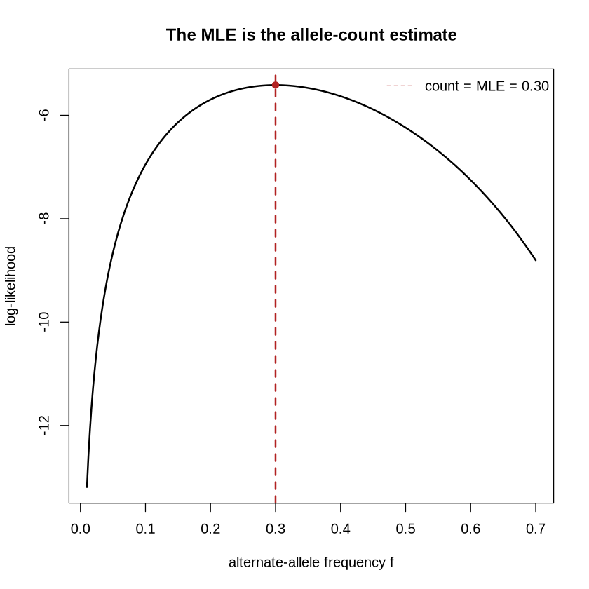
Plot with title “The MLE is the allele-count estimate”

Insight behind the approach¶

HWE gives a probabilistic model for the true genotype given allele frequency. Changing $f$ changes the expected genotype frequencies along the HWE curve. Genotyping error changes the observed calls in a different pattern. Likelihood uses these patterns to estimate both $f$ and the error rate.

3. Genotyping error separates genotype from measurement¶

The true genotype $G_i$ is a biological state. The observed genotype call $D_i$ is produced by measurement and genotype calling. The model connects them in two steps.

f \longrightarrow G_i \longrightarrow D_i.

(5)

The HWE model gives the probability of $G_i$ from $f$ .
The measurement model gives the probability of $D_i$ from $G_i$ . With probability $\epsilon$ , the calling process makes an error event and assigns one of the three calls at random. Thus

P(D_i=d\mid G_i=g,\epsilon)= \begin{cases} 1-2\epsilon/3, & d=g,\\ \epsilon/3, & d\ne g. \end{cases}

(6)

This simple error model keeps the calculation visible. A sequencing analysis can use read-level genotype likelihoods in place of this call-error matrix.

# Simulation with known truth.
set.seed(581)
f_true <- 0.30
epsilon_true <- 0.05
n <- 10000

g_true <- sample(0:2, n, replace = TRUE, prob = hwe_prob(f_true))
d_observed <- g_true
error_event <- runif(n) < epsilon_true
d_observed[error_event] <- sample(0:2, sum(error_event), replace = TRUE)

observed_counts <- table(factor(d_observed, levels = 0:2))
n <- length(d_observed)

f_observed_count <- sum(d_observed) / (2 * n)

data.frame(observed_call = 0:2, count = as.integer(observed_counts))
cat(sprintf("True MAF: %.3f\n", f_true))
cat(sprintf("Direct count of observed calls: %.3f\n", f_observed_count))
cat(sprintf("Simulated error events: %d of %d\n", sum(error_event), n))

True MAF: 0.300

Direct count of observed calls: 0.313

Simulated error events: 494 of 10000

HWE gives a diagnostic for genotype measurement error¶

Under HWE, the three true genotype probabilities are determined by one parameter $f$ .

\mathbf p(f)=\left((1-f)^2,\;2f(1-f),\;f^2\right).

(7)

As $f$ changes, these probabilities trace a one-dimensional HWE curve. Under the simple error model used here, the observed-call probability is

q_d(f,\epsilon)=(1-\epsilon)p_d(f)+\frac{\epsilon}{3}.

(8)

Changing $f$ moves the genotype probabilities along the HWE curve. Increasing $\epsilon$ pulls the observed-call probabilities toward $(1/3,1/3,1/3)$ , which generally moves them away from the HWE curve. The two parameters therefore leave different patterns in the three genotype counts.

A practical diagnostic fits HWE using the allele-count estimate and compares the observed and expected genotype counts. Departure from HWE signals model mismatch. Genotyping error is one possible explanation. Population structure, inbreeding, and selection can also produce departure from HWE.

hwe_expected <- n * hwe_prob(f_observed_count)
hwe_residual <- (as.numeric(observed_counts) - hwe_expected) /
  sqrt(hwe_expected)

hwe_diagnostic <- data.frame(
  genotype_call = 0:2,
  observed = as.integer(observed_counts),
  expected_under_HWE = round(hwe_expected, 1),
  Pearson_residual = round(hwe_residual, 2)
)

hwe_chisq <- sum(hwe_residual^2)
hwe_p <- pchisq(hwe_chisq, df = 1, lower.tail = FALSE)

hwe_diagnostic
cat(sprintf(
  "HWE diagnostic. X^2 = %.2f, df = 1, p = %s\n",
  hwe_chisq, format.pval(hwe_p, digits = 3)
))

HWE diagnostic. X^2 = 8.68, df = 1, p = 0.00322

In this simulation, the observed genotype calls depart from the fitted HWE expectation. The error-aware model adds a measurement process. It treats the true genotype as latent and sums over its three possible values. The simulated true genotypes are retained only to check the answer.

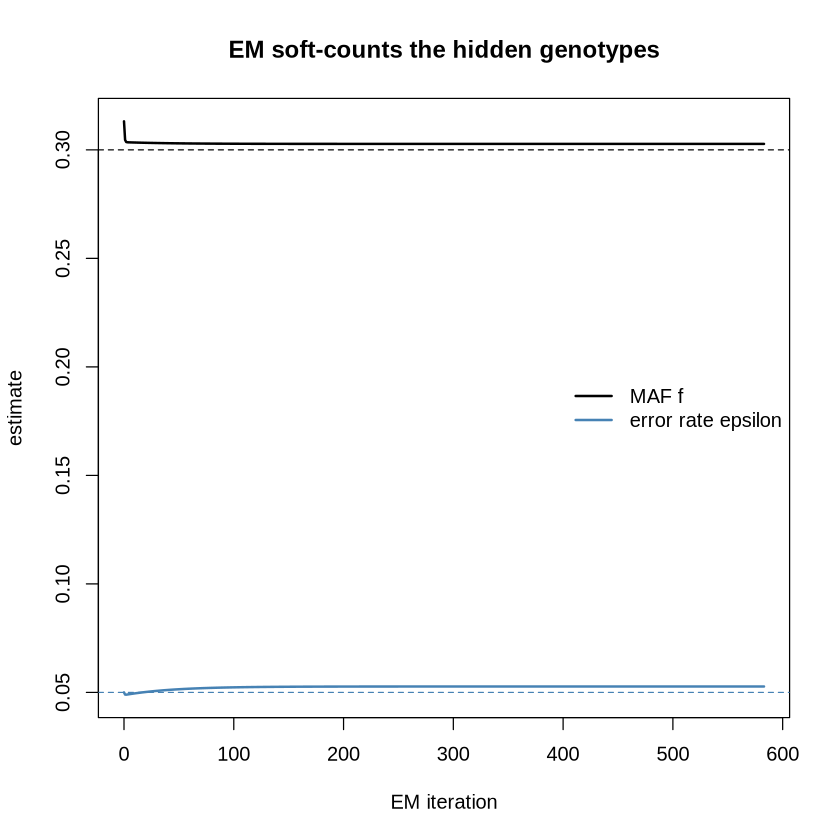
L(f,\epsilon)=\prod_{i=1}^n\sum_{g=0}^2 P(D_i=d_i\mid G_i=g,\epsilon)P(G_i=g\mid f).

(9)

EM applies this calculation to every person through repeated soft counting.

E-step infers each hidden genotype¶

w_{ig}=P(G_i=g\mid D_i=d_i,f,\epsilon) \propto P(D_i=d_i\mid G_i=g,\epsilon)P(G_i=g\mid f).

(10)

M-step recounts expected alleles and errors¶

f^{\text{new}}=\frac{1}{2n}\sum_i(w_{i1}+2w_{i2}),\qquad \epsilon^{\text{new}}=\frac{3}{2n}\sum_i[1-w_{i,d_i}].

(11)

The key idea is simple. Replace each hidden genotype by posterior weights, then count with those weights.

error_matrix <- function(epsilon) {
  out <- matrix(epsilon / 3, 3, 3,
                dimnames = list(observed = 0:2, true = 0:2))
  diag(out) <- 1 - 2 * epsilon / 3
  out
}

joint_genotype_prob <- function(d, f, epsilon) {
  error_matrix(epsilon)[d + 1, , drop = FALSE] *
    rep(hwe_prob(f), each = length(d))
}

genotype_weights <- function(d, f, epsilon) {
  joint <- joint_genotype_prob(d, f, epsilon)
  joint / rowSums(joint)
}

observed_loglik <- function(d, f, epsilon) {
  sum(log(rowSums(joint_genotype_prob(d, f, epsilon))))
}

em_update <- function(d, f, epsilon) {
  weight <- genotype_weights(d, f, epsilon)
  expected_dosage <- as.numeric(weight %*% (0:2))
  posterior_match <- weight[cbind(seq_along(d), d + 1)]
  c(
    f = mean(expected_dosage) / 2,
    epsilon = min(1 - 1e-10, 1.5 * mean(1 - posterior_match))
  )
}

fit_em <- function(d, f = mean(d) / 2, epsilon = 0.05,
                   tolerance = 1e-10, max_iterations = 10000) {
  history <- data.frame(
    iteration = 0, f = f, epsilon = epsilon,
    loglik = observed_loglik(d, f, epsilon)
  )

  for (iteration in seq_len(max_iterations)) {
    updated <- em_update(d, f, epsilon)
    f_new <- updated[["f"]]
    epsilon_new <- updated[["epsilon"]]
    history <- rbind(history, data.frame(
      iteration = iteration, f = f_new, epsilon = epsilon_new,
      loglik = observed_loglik(d, f_new, epsilon_new)
    ))

    change <- max(abs(c(f_new - f, epsilon_new - epsilon)))
    f <- f_new
    epsilon <- epsilon_new
    if (change < tolerance) break
  }

  list(
    f = f, epsilon = epsilon,
    posterior = genotype_weights(d, f, epsilon),
    history = history
  )
}

em_fit <- fit_em(d_observed)

data.frame(
  parameter = c("MAF f", "error rate epsilon"),
  truth = c(f_true, epsilon_true),
  direct_count = c(f_observed_count, NA),
  EM = c(em_fit$f, em_fit$epsilon)
)

tail(em_fit$history, 5)

posterior_by_call <- cbind(
  observed_call = 0:2,
  genotype_weights(0:2, em_fit$f, em_fit$epsilon)
)
colnames(posterior_by_call) <- c("observed_call",
                                 "P(true=0)", "P(true=1)", "P(true=2)")
round(posterior_by_call, 4)

matplot(em_fit$history$iteration,
        em_fit$history[, c("f", "epsilon")],
        type = "l", lty = 1, lwd = 2,
        col = c("black", "steelblue"),
        xlab = "EM iteration", ylab = "estimate",
        main = "EM soft-counts the hidden genotypes")
abline(h = c(f_true, epsilon_true), lty = 2,
       col = c("black", "steelblue"))
legend("right", legend = c("MAF f", "error rate epsilon"),
       col = c("black", "steelblue"), lty = 1, lwd = 2, bty = "n")

Plot with title “EM soft-counts the hidden genotypes”

4. Check the answer two ways¶

Direct optimization of the same observed-data likelihood should agree with EM. The observed-data log-likelihood should also increase or remain unchanged at every EM iteration.

negative_loglik <- function(par, d) {
  -observed_loglik(d, f = par["f"], epsilon = par["epsilon"])
}

direct_fit <- optim(
  par = c(f = 0.30, epsilon = 0.05),
  fn = negative_loglik,
  d = d_observed,
  method = "L-BFGS-B",
  lower = c(1e-6, 1e-6),
  upper = c(0.5 - 1e-6, 1 - 1e-6)
)

comparison <- data.frame(
  parameter = c("MAF f", "error rate epsilon"),
  truth = c(f_true, epsilon_true),
  EM = c(em_fit$f, em_fit$epsilon),
  direct_optimization = direct_fit$par
)
comparison$difference <- comparison$EM - comparison$direct_optimization
comparison

stopifnot(direct_fit$convergence == 0)
stopifnot(max(abs(comparison$difference)) < 1e-4)
stopifnot(all(diff(em_fit$history$loglik) >= -1e-8))
cat("Checks passed: EM agrees with direct optimization, and likelihood is monotone.\n")

Checks passed: EM agrees with direct optimization, and likelihood is monotone.

What to remember¶

Concept and intuition. Allele frequency counts chromosome copies. Sequencing provides measurements from which genotypes are inferred.
Insight behind the approach. HWE restricts the three genotype frequencies to a one-parameter curve. Genotyping error generally moves the observed-call frequencies away from that curve. These different patterns let likelihood estimate both $f$ and $\epsilon$ .
Worked example. An HWE comparison detects model mismatch. The error-aware model then uses EM to recover the MAF and error rate, with direct likelihood optimization as a check.

The error-aware estimate is useful when the error model describes the measurement process.

Source record and further detail¶

The genotyping-error simulation uses seed 581, $n=10{,}000$ , true MAF 0.30, and true error rate 0.05. The result is checked by direct likelihood optimization.
Pritchard, An Owner’s Guide to the Human Genome, Chapter 1.3, especially allele frequency, genotype coding, and HWE.