A first EM algorithm - P8149 Computational Vignettes

When EM applies¶

EM applies when two easy problems depend on each other.

If the hidden variable $Z$ were known, estimating $\theta$ would be easy.
If $\theta$ were known, calculating $p(Z\mid X,\theta)$ would be easy.

EM solves them in turn.

E step. Use the current $\theta$ to calculate probabilities for $Z$ .
M step. Use those probabilities to update $\theta$ .

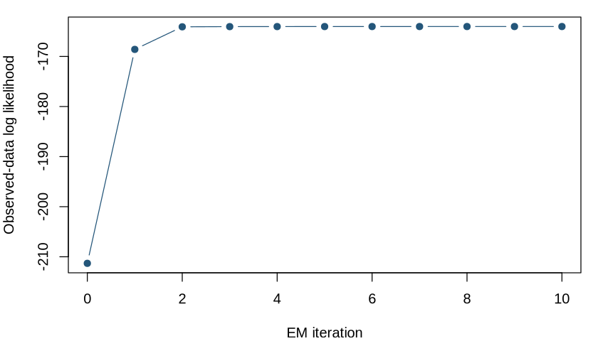
Then repeat. Each round raises or preserves the observed-data likelihood. The iteration converges to a stationary point, although the point can depend on the starting values.

This requires a joint model $p(X,Z\mid\theta)$ and E and M steps that we can compute.

A two-group model¶

We observe $X_i$ , but not its group $Z_i$ . If the group labels were known, the group proportions and means would be simple counts and averages. EM calculates a probability for each label and uses those probabilities as weights.

Let $P(Z_i=1)=\pi$ and

X_i\mid Z_i=k\sim N(\mu_k,1),\qquad k\in\{0,1\}.

(1)

The unknown parameters are $\theta=(\pi,\mu_0,\mu_1)$ .

One fixed sample¶

We simulate one observed value from one of two hidden groups. The hidden label is shown because this is a teaching example. In real data, it is unknown. The observed value could, for example, be an apple weight and the hidden label its variety.

set.seed(8149)

n_sample <- 80L
hidden_group <- sample(rep(c(0, 1), each = n_sample / 2))
true_mean <- c(-1.5, 1.5)
observed <- rnorm(
  n_sample, mean = true_mean[hidden_group + 1], sd = 1
)

data.frame(
  observed = round(observed[1:8], 2),
  hidden_group = hidden_group[1:8]
)

Loading...

E step: infer the hidden group¶

Given the current parameters, calculate the probability that observation $i$ came from group 1.

r_i^{(t)} =P(Z_i=1\mid X_i=x_i,\theta^{(t)}) =\frac{\pi^{(t)}\phi(x_i;\mu_1^{(t)},1)} {(1-\pi^{(t)})\phi(x_i;\mu_0^{(t)},1) +\pi^{(t)}\phi(x_i;\mu_1^{(t)},1)}.

(2)

$r_i^{(t)}$ is also $E[Z_i\mid X_i,\theta^{(t)}]$ . It is the expected group-1 count contributed by observation $i$ .

responsibility <- function(observed, pi, mu) {
  density_0 <- (1 - pi) * dnorm(observed, mean = mu[1], sd = 1)
  density_1 <- pi * dnorm(observed, mean = mu[2], sd = 1)
  density_1 / (density_0 + density_1)
}

start <- list(pi = 0.5, mu = c(-0.5, 0.5))
r <- responsibility(observed, start$pi, start$mu)
ordered <- order(observed)

options(repr.plot.width = 7, repr.plot.height = 4)
par(mar = c(4, 4, 1, 1))
plot(
  observed[ordered], r[ordered], type = "b", pch = 19,
  xlab = "Observed value",
  ylab = "P(hidden group = 1 | observed value)",
  ylim = c(0, 1), col = "#24567a"
)
abline(h = 0.5, lty = 2, col = "#7a8793")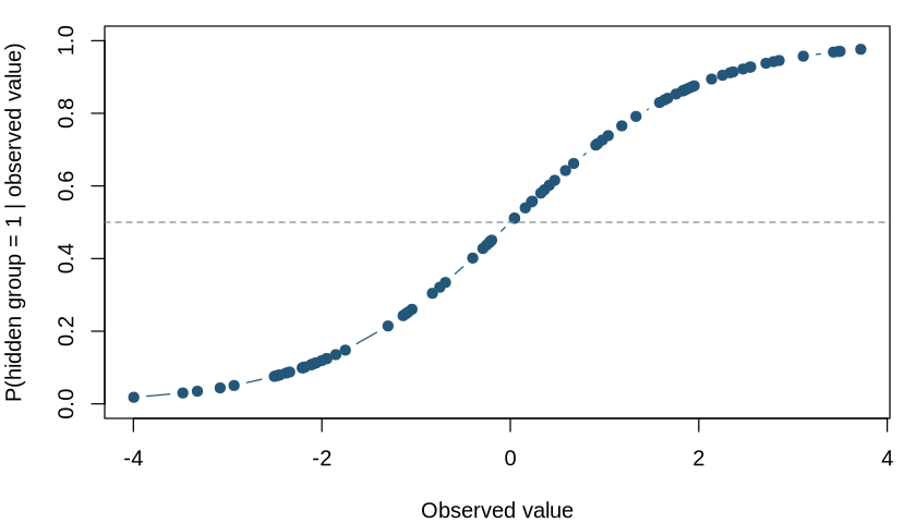

A responsibility is not a hard group label. It measures uncertainty about the hidden group. Values near $1/2$ mean that the two groups remain difficult to distinguish.

M step: update the parameters¶

Use the responsibilities as fractional group labels.

\pi^{(t+1)}=\frac{1}{n}\sum_i r_i^{(t)},

(3)

\mu_0^{(t+1)}=\frac{\sum_i(1-r_i^{(t)})x_i}{\sum_i(1-r_i^{(t)})},\qquad \mu_1^{(t+1)}=\frac{\sum_i r_i^{(t)}x_i}{\sum_i r_i^{(t)}}.

(4)

In general, the M step maximizes the expected complete-data log likelihood.

\theta^{(t+1)}=\arg\max_{\theta} E_{Z\mid X,\theta^{(t)}}\left[\ell_c(\theta;X,Z)\right].

(5)

observed_loglik <- function(observed, pi, mu) {
  density <-
    (1 - pi) * dnorm(observed, mean = mu[1], sd = 1) +
    pi * dnorm(observed, mean = mu[2], sd = 1)
  sum(log(density))
}

em_update <- function(observed, pi, mu) {
  r <- responsibility(observed, pi, mu)
  list(
    pi = mean(r),
    mu = c(
      sum((1 - r) * observed) / sum(1 - r),
      sum(r * observed) / sum(r)
    )
  )
}

fit_em <- function(observed, start, tolerance = 1e-8) {
  parameter <- start
  history <- data.frame(
    iteration = 0L, pi = parameter$pi,
    mu_0 = parameter$mu[1], mu_1 = parameter$mu[2],
    loglik = observed_loglik(observed, parameter$pi, parameter$mu)
  )

  for (iteration in seq_len(500L)) {
    updated <- em_update(observed, parameter$pi, parameter$mu)
    change <- max(abs(
      c(updated$pi, updated$mu) - c(parameter$pi, parameter$mu)
    ))
    parameter <- updated
    history <- rbind(
      history,
      data.frame(
        iteration = iteration, pi = parameter$pi,
        mu_0 = parameter$mu[1], mu_1 = parameter$mu[2],
        loglik = observed_loglik(
          observed, parameter$pi, parameter$mu
        )
      )
    )
    if (change < tolerance) break
  }

  parameter$history <- history
  parameter
}

fit <- fit_em(observed, start)

Why the iteration works¶

The observed-data log likelihood contains a sum over the hidden variable.

\ell(\theta;X)=\log\sum_Z p(X,Z\mid\theta).

(6)

After the E step, let $q_t(Z)=p(Z\mid X,\theta^{(t)})$ . This distribution gives every possible hidden assignment a weight. With these weights fixed, EM uses the bound

\mathcal F(q_t,\theta) =E_{q_t}[\log p(X,Z\mid\theta)]+H(q_t) \leq \ell(\theta;X).

(7)

$H(q_t)=-E_{q_t}[\log q_t(Z)]$ measures the remaining uncertainty about the hidden assignment. It is constant during the M step. The bound touches the observed-data log likelihood at the current parameters. The M step raises the bound, and the new likelihood lies above the new bound.

\ell(\theta^{(t+1)};X) \geq \mathcal F(q_t,\theta^{(t+1)}) \geq \mathcal F(q_t,\theta^{(t)}) =\ell(\theta^{(t)};X).

(8)

Any valid initial value can start the iteration. Under the usual regularity conditions, the likelihood converges and the parameter estimates approach a stationary point. Different initial values can reach different stationary points, so a useful starting value can still matter.

data.frame(
  parameter = c("pi", "mu_0", "mu_1"),
  true_value = c(0.5, true_mean),
  estimate = round(c(fit$pi, fit$mu), 3)
)

stopifnot(all(diff(fit$history$loglik) >= -1e-10))

shown <- fit$history[fit$history$iteration <= 10, ]
options(repr.plot.width = 7, repr.plot.height = 4)
par(mar = c(4, 4, 1, 1))
plot(
  shown$iteration, shown$loglik,
  type = "b", pch = 19, col = "#24567a",
  xlab = "EM iteration", ylab = "Observed-data log likelihood"
)

Loading...

What to remember¶

EM applies when hidden data would make estimation simple and both the E and M steps can be computed.
The E step turns each hidden value into a probability. The M step uses those probabilities as fractional observations.
Each iteration raises or preserves the observed-data likelihood, but different starting values can lead to different stationary points.

The genotyping-error model uses the same structure. The latent variable is the true genotype, and the observed data are uncertain genotype measurements.