Getting Started#
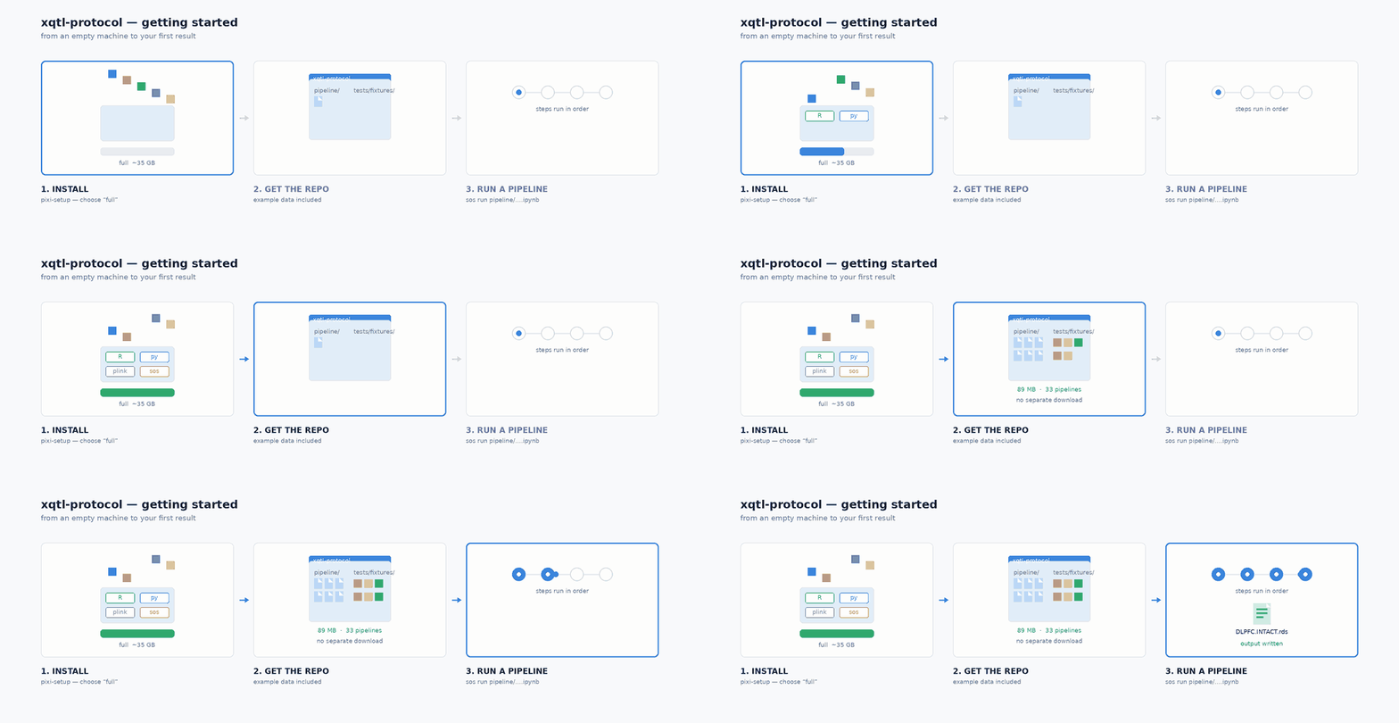
Three steps take you from an empty machine to your first pipeline run:
Step |
What it does |
|---|---|
1. Install the environment |
|
2. Get the repo |
the example data comes with it — no separate download |
3. Run a pipeline |
|
Not sure which pipelines you need? Use the pipeline selector. Answer a few questions about your data — molecular phenotype, whether you are fine-mapping from individual-level data or summary statistics, whether you are integrating with GWAS — and it lists the pipelines that apply, with their inputs, outputs and the commands to run them. This page covers how to run a pipeline; the selector tells you which.
Before You Start#
The protocol’s pipelines are written as SoS (Script of Scripts) workflows. You do not need to install SoS separately — it comes with the environment in Step 1, along with a registered sos Jupyter kernel if you would rather work interactively.
Native support is provided for Linux and macOS (Intel and Apple Silicon). Windows users need WSL.
Step 1. Install the xQTL Software Stack with pixi#
Install the bioinformatics and data-science packages the protocol depends on using pixi via the StatFunGen/pixi-setup installer. Full reference: Advanced Software Setup with Pixi.
On HPC systems, your home directory likely has a storage quota that will not fit the full install. Point HOME at a path with enough space, and add pixi to your $PATH:
# Point HOME to a location with enough disk space
export HOME="/your_pixi_install_path"

# Add pixi to your path
export PATH="/your_pixi_install_path/.pixi/bin:$PATH"
Then download the installer and run it:
curl -fsSL https://raw.githubusercontent.com/StatFunGen/pixi-setup/refs/heads/main/pixi-setup.sh -o pixi-setup.sh
bash pixi-setup.sh
On a laptop or workstation you can skip the HOME/PATH exports and just run the two commands above — the installer will prompt you to choose an install path.
The installer will prompt you for two things:
1. Installation path — where pixi stores environments and packages.
Setting |
When to use |
|---|---|
|
Laptops and workstations with plenty of home-directory space |
|
HPC systems with strict home-directory quotas |
2. Installation type
Type |
Size |
Files |
Includes |
|---|---|---|---|
1. minimal |
~5 GB |
~100k |
CLI tools, Python data-science stack, JupyterLab, base R (tidyverse, devtools, IRkernel) |
2. full |
~35 GB |
~350k |
Everything above, plus the bioinformatics suite — plink, samtools, bcftools, bedtools, STAR, GATK4, tensorqtl, Seurat, Bioconductor packages |
Choose full for this protocol; minimal does not include the bioinformatics tools the pipelines call.
Then restart your shell, or:
source ~/.bashrc
Verify:
which sos Rscript        # both should resolve inside your pixi install
sos --version
jupyter kernelspec list  # should include 'sos'
Step 2. Clone the Protocol#
git clone https://github.com/StatFunGen/xqtl-protocol.git
cd xqtl-protocol
Run everything from the root of the repository. All pipelines are symbolic links in the pipeline folder, so you execute them directly as sos run pipeline/<pipeline_file>.ipynb.
Step 3. The Example Data#
You do not need to download anything. Example data is included in this repository under tests/fixtures/ — about 89 MB covering 33 pipelines:
ls tests/fixtures/
apa_calling   gwas_qc   intact   mash   pca   rna_calling   twas   vcf_qc
qtl_mini      sldsc_enrichment    splicing_calling   susie_enloc   ...
Each directory holds the inputs for one pipeline, sized down to chromosome 22 so a pipeline runs in minutes. Some directories also carry reference data — genome annotation, LD panels — under their upstream filenames so you can see where they came from.
To run a pipeline on your own data, pass your own file paths to the same parameters in place of the tests/fixtures/… ones.
Step 4. Run Your First Pipeline#
Add -n to preview first: SoS parses the notebook, binds your parameters, prints the command it would run, and touches no data. It takes seconds, so it is a good habit before a long job.
sos run pipeline/intact.ipynb intact \\
    --fastenloc-file tests/fixtures/intact/protocol_example.fastenloc.gene.out \\
    --ptwas-file     tests/fixtures/intact/protocol_example.ptwas.output \\
    --tissue DLPFC --cwd /tmp/intact_demo -n
Then drop the -n to run it:
INFO: intact output: /tmp/intact_demo/DLPFC.INTACT.rds
Two shapes of pipeline#
Inputs passed directly — as above, point straight at files in tests/fixtures/.
Inputs staged into a working directory — some pipelines look for *.gz inside their --cwd rather than taking file arguments, so copy the example data in first:
W=/tmp/qtlpp; mkdir -p $W/tensorqtl_cis $W/out
cp tests/fixtures/qtl_association_postprocessing/*.gz $W/tensorqtl_cis/

sos run pipeline/qtl_association_postprocessing.ipynb default \\
    --cwd $W/tensorqtl_cis --modular-script-dir code/script --output-dir $W/out \\
    --maf-cutoff 0.01 --cis-window 1000000 --pvalue-cutoff 0.05 \\
    --study protocol_example --context bulk_rnaseq --genome hg38
Finding the parameters for any pipeline#
Each pipeline’s tests carry parameter sets that are known to work, which is the quickest way to get a runnable command for one you have not used before:
# which test drives the notebook you want
grep -rl 'run_sos' tests/notebooks --include='*.py'

# the notebook, step and parameters
grep -n -A16 'run_sos(' tests/notebooks/<path>/test_<name>.py
Translating what you find into command-line flags: output_prefix="toy" becomes --output-prefix toy, fx / "twas/protocol_example.x.tsv" becomes tests/fixtures/twas/protocol_example.x.tsv, and repo_root / "code/script" becomes --modular-script-dir code/script.
Next, the Analysis section below indexes every pipeline in the protocol, roughly upstream to downstream.
Analysis#
Please visit the homepage of the protocol website for the general background on this resource, in particular the How to use the resource section. To perform a complete analysis from molecular phenotype quantification to xQTL discovery, conduct your analysis in the order listed below. Each link contains a mini-protocol for a specific task, and all commands should be executed from the command line.
Important
Minimum Working Example — new users, start here.
Every module ships a minimal test dataset (prefixed with MWE) under Synapse syn69670658. To go end-to-end on the demo data, run these five pipelines in order and skip everything else on the first pass:
reference_data.ipynb— prepare standardized reference filesbulk_expression.ipynb— quantify gene expressiongenotype_preprocessing.ipynb→phenotype_preprocessing.ipynb→covariate_preprocessing.ipynb— QC and normalizationqtl_association_testing.ipynb— cis-QTL with TensorQTLmnm_miniprotocol.ipynb— fine-mapping + TWAS with SuSiE
Once this pass completes, branch out to the additional modules below based on what your project needs.
1. Reference Data#
Multiple reference data files are required before molecular phenotypes are quantified — reference genomes, gene annotations, variant annotations, linkage disequilibrium data and topologically associated domains.
Reference data — overview and required input files ⭐ MWE
Reference data preparation — downloading and standardizing reference files
Generalized TAD boundaries — topologically associating domain annotations
LD reference pruning — pruned LD reference panels
RSS LD sketching — LD matrix sketches for summary-statistics methods
2. Molecular Phenotype Quantification#
Molecular phenotypic data is required for the generation of QTLs. We support bulk RNA-Seq, methylation, splicing and alternative-polyadenylation (APA) phenotypes. Quantification of gene expression is conducted with either RNA-SeQC for gene-level counts, or RSEM for transcript-level counts. Quantification of alternative splicing events is conducted with leafcutter2 to identify alternatively excised introns. Quantification of DNA methylation is done using SeSAMe. Each phenotype then undergoes phenotype-specific quality control and normalization.
Gene expression (RNA-seq) — RNA-SeQC or RSEM ⭐ MWE
Alternative splicing — leafcutter2
DNA methylation — SeSAMe
Alternative polyadenylation (APA) — DaPars2
3. Data Pre-Processing#
Preprocessing of genotype data begins with the application of variant filters using bcftools. VCF files are then converted to plink format so that kinship analyses may be performed to identify unrelated individuals. Genetic principal components are then generated for unrelated samples and genotype files are formatted for QTL analysis. Preprocessing of phenotypic data begins with annotation of features, followed by imputation of missing entries and formatting. Preprocessing of covariates merges phenotypic data with genetic principal components, then computes hidden factors to use as additional covariates.
4. QTL Association Testing#
QTL association analysis is conducted with TensorQTL. We include options for cis or trans analysis, with options to include interaction terms. Hierarchical multiple testing may then be applied to adjust p-values.
QTL association testing ⭐ MWE
TensorQTL — cis/trans scans with optional interaction terms
Quantile regression QTL & TWAS — non-linear genotype-phenotype effects
Association post-processing — hierarchical multiple testing correction
5. Multivariate Mixture Model#
For multi-context or multi-tissue analyses, we provide a multivariate mixture model framework based on MASH. This learns a data-driven mixture prior across contexts and estimates effect sizes and posterior probabilities for sharing of eQTLs across tissues.
Multivariate mixture vignette — overview and walkthrough
Mixture prior estimation (MASH) — learn data-driven covariance matrices
MASH model fitting — fit the model and compute posterior summaries
6. Multiomics Regression Models (Fine-mapping)#
Our pipeline includes multiple methods for fine-mapping of QTLs. Univariate fine-mapping and TWAS with SuSiE generates TWAS weights and credible sets. Regression with summary statistics allows inclusion of GWAS summary stats in SuSiE fine-mapping. Univariate fine-mapping of functional data uses epigenomic annotations with fSuSiE.
7. GWAS Integration#
We include methods for colocalization analysis, starting with the generation of prior probabilities followed by pairwise colocalization of xQTL and GWAS fine-mapping results to identify shared causal variants. We also include TWAS and cTWAS to identify genes associated with complex traits.
Colocalization (SuSiE-enloc) — pairwise xQTL-GWAS colocalization
TWAS & cTWAS — genes associated with complex traits
ColocBoost — shared-variant discovery across molecular traits
8. Enrichment and Validation#
We utilize an excess of overlap method to evaluate the enrichment of significant variants within specific genomic annotations. Pathway enrichment analysis identifies biological pathways that are statistically overrepresented in a given gene set. Stratified LD Score Regression (S-LDSC) quantifies the contribution of genomic functional annotations to heritability of complex traits. By integrating GWAS summary statistics with genome annotations, S-LDSC distinguishes true polygenic signals from confounding effects.
Excess-of-overlap enrichment — variant enrichment in genomic annotations
Gene set enrichment (GSEA) — overrepresented biological pathways
GREGOR — annotation-based enrichment for regulatory variants
Stratified LD Score Regression — heritability partitioning by annotation
9. xQTL Modifier Score (EMS)#
The xQTL modifier score framework trains a per-variant model for prioritizing regulatory variants.
EMS training — fit the model using functional annotation features
EMS prediction — score new variants
10. Command Generator#
eQTL analysis command generator — produce full pipeline commands from a single configuration file
Software Environment#
Every protocol on this site runs inside the pixi environment configured in Steps 1-2. Once pixi and SoS are installed, each example “just works” — no per-pipeline container, no manual dependency wrangling.
Need something extra? Install it into the right pixi environment:
# Python package (into the shared python env)
pixi global install -c conda-forge --environment python <package>

# R package (into the r-base env)
pixi global install -c conda-forge --environment r-base r-<package>

# Standalone bioinformatics CLI tool
pixi global install -c bioconda <tool>
Troubleshooting#
Warning
R library conflicts. If you see an error like
Error in dyn.load(file, DLLpath = DLLPath, ...):
unable to load shared object '$PATH/R/x86_64-pc-linux-gnu-library/4.2/stringi/libs/stringi.so':
libicui18n.so.63: cannot open shared object file: No such file or directory
your system R libraries are being picked up alongside the pixi ones. Unset them before running the pipeline:
export R_LIBS=""
export R_LIBS_USER=""
pixi: command not found — open a new terminal, or re-source your shell rc file (source ~/.bashrc on Linux/HPC, source ~/.zshrc on macOS).
Installer killed on HPC — you’re on a login node. Request a compute node with ≥ 50 GB memory and re-run.
sos: command not found — Step 1 didn’t complete. Re-run the conda install command for SoS.
ModuleNotFoundError during a pipeline — install the missing package into pixi’s python env with the command above.
Still stuck? Open an issue with the command you ran and the full error output.
Analyses on High Performance Computing Clusters#
The demo on this page runs on a desktop workstation. Production analyses typically run on an HPC cluster, and SoS supports this natively via SoS Remote Tasks on configured host computers.
We provide a toy example for running SoS pipelines on a typical HPC cluster environment — first-time users are encouraged to work through it before launching real jobs. It covers the host and task configuration you’ll reuse for every subsequent pipeline, and it’s schedule-agnostic (SLURM, LSF, SGE, PBS/Torque all work).