Collider#
A collider is a variable that is influenced by two other variables of interest, creating a spurious association between them when we condition on (select or control for) the collider in our analysis.
Graphical Summary#
Key Formula#
The key formula for the concept of a collider is represented in a causal diagram as:
Where:
\(W\) is the collider variable
\(X\) is one cause of the collider
\(Y\) is another cause of the collider
The arrows (\(\rightarrow\)) indicate the direction of causal influence
This diagram illustrates that a collider (\(W\)) is a variable that is caused by both the exposure (\(X\)) and the outcome (\(Y\)), creating a situation where \(X\) and \(Y\) both flow into \(W\).
When we condition on (adjust for, stratify by, or select based on) a collider, we can induce a spurious association between its causes, even if they were originally independent.
Technical Details#
What Happens When We Control for Colliders#
When a collider is present and incorrectly controlled for:
True Effect: The real biological relationship (may be zero)
Collider Bias: The false association created by conditioning on the collider
Observed Association: What we measure after incorrectly adjusting (often misleading!)
The Problem: Conditioning on Colliders Creates Bias#
Unlike confounders, colliders should NOT be included in regression models. Including a collider as a covariate can create spurious associations:
This regression will give a biased estimate of \(\beta_1\) even when the true effect is zero.
Why This Happens: Selection Bias#
Controlling for a collider creates selection bias by conditioning on a variable that depends on both exposure and outcome:
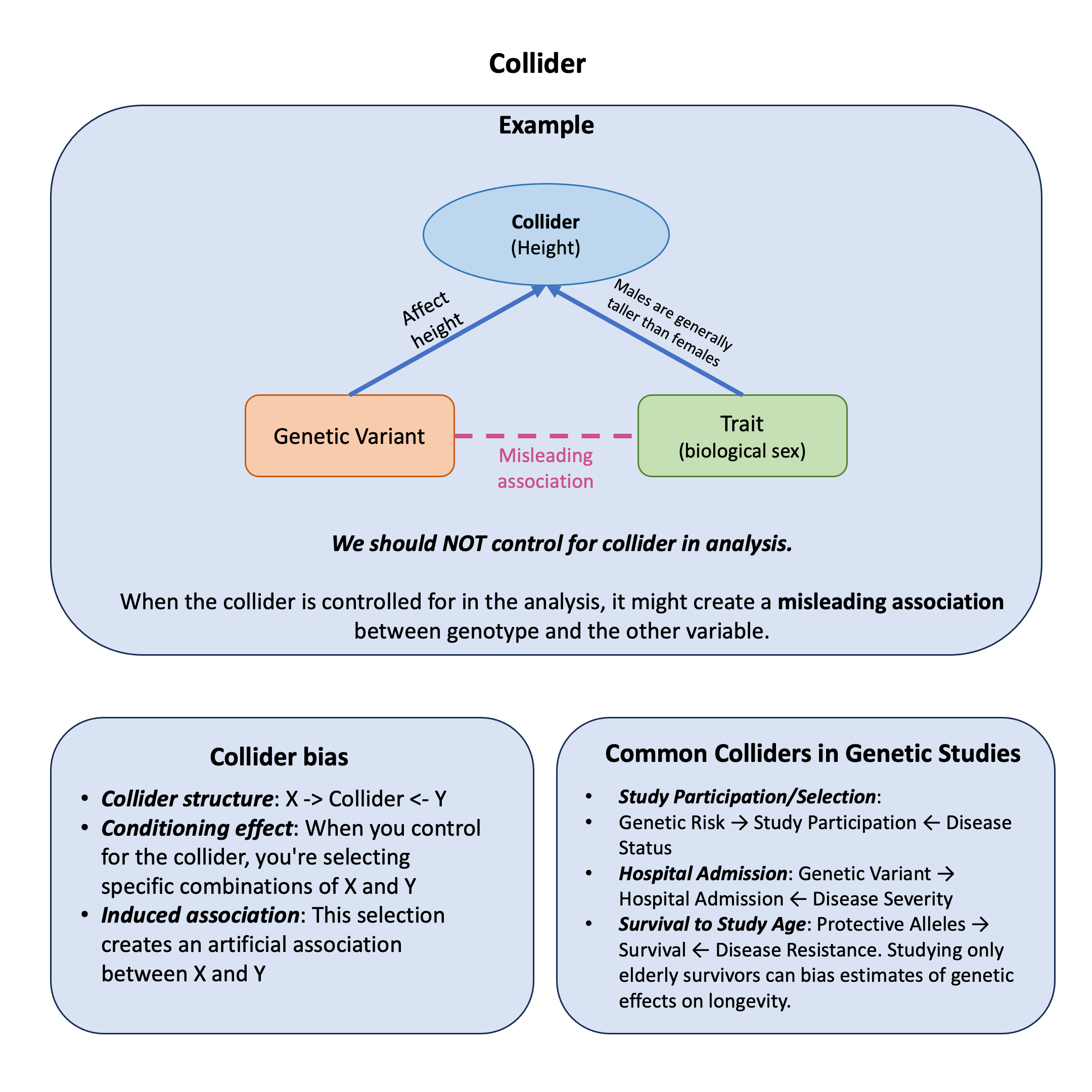
Collider structure: \(X \rightarrow \text{Collider} \leftarrow Y\)
Conditioning effect: When you control for the collider, you’re selecting specific combinations of X and Y
Induced association: This selection creates an artificial association between X and Y
Common Colliders in Genetic Studies#
Study Participation/Selection: Genetic Risk \(\leftarrow\) Study Participation \(\rightarrow\) Disease Status
Hospital Admission: Genetic Variant \(\leftarrow\) Hospital Admission \(\rightarrow\) Disease Severity
Survival to Study Age: Protective Alleles \(\leftarrow\) Survival \(\rightarrow\) Disease Resistance. Studying only elderly survivors can bias estimates of genetic effects on longevity.
The Key Principle#
Confounders: Control to remove bias
Colliders: Don’t control to avoid creating bias
Example#
Here’s a biologically implausible scenario that perfectly demonstrates collider bias: What if we told you that certain genetic variants (autosomal SNPs) are associated with biological sex? That sounds absurd, right? Sex is determined by sex chromosomes (XX or XY), so autosomal SNPs (variants on non-sex chromosomes) should have zero association with whether someone is male or female.
Yet, if we make one seemingly innocent analytical choice—adjusting for height in our model—we can create hundreds of “genome-wide significant” associations between autosomal SNPs and sex. These associations are completely spurious, arising purely from collider bias.
This example is based on a landmark study published in the American Journal of Human Genetics that used UK Biobank data to definitively demonstrate collider bias. The researchers deliberately induced this bias to show how adjusting for heritable covariates can create biologically impossible associations.
The Setup: Height as a Collider#
The causal structure is:
Genetic variants influence height (taller alleles exist)
Sex influences height (males are typically taller than females)
SNPs and sex are causally independent (autosomal variants don’t cause sex)
Height is the collider—it’s caused by both SNP and sex
When we condition on height (e.g., by only studying tall people, or by including height as a covariate), we induce a spurious association between SNPs and sex, even though no biological relationship exists.
Why Does This Create Bias?#
Think about it this way: If you restrict your analysis to very tall people, you’re selecting a group where:
Females with height-increasing alleles are more likely to be included
Males without height-increasing alleles are more likely to be included
This creates an artificial negative correlation: within tall people, having height-increasing alleles makes you more likely to be female. But this correlation exists only because we conditioned on height, not because of any biological relationship between autosomal SNPs and sex.
Let’s demonstrate this with a simulation.
Simulation Setup#
We’ll create data for 10,000 individuals where we know the true relationships. We’ll simulate:
Sex (independent, ~50% male/female)
A genetic variant (SNP) that affects height (independent of sex)
Height, which is influenced by both sex and the SNP
rm(list=ls())
set.seed(123)

# Sample size
N <- 10000

# Generate sex (0 = Female, 1 = Male)
# Sex is randomly assigned and independent of genetics
sex <- rbinom(N, 1, 0.5)

# Generate SNP (0, 1, 2 copies of a height-increasing allele)
# This is a common autosomal variant, independent of sex
snp <- sample(0:2, N, replace = TRUE, prob = c(0.25, 0.5, 0.25))
Now we build the causal relationships that make height a collider. Height is influenced by both sex and the genetic variant, but sex and the SNP are causally independent:
# Height is caused by BOTH sex and SNP
# Males are on average 13 cm taller
# Each copy of the height-increasing allele adds ~2 cm
height_cm <- 160 +           # Baseline (female, 0 copies)
             13 * sex +       # Sex effect (males taller)
             2 * snp +        # SNP effect (each allele adds height)
             rnorm(N, 0, 6)   # Individual variation
Analysis 1: Correct Approach (No Adjustment for Height)#
First, let’s test the association between SNP and sex without adjusting for height. Since autosomal SNPs don’t cause sex, we should see no association:
# Standardize variables for easier interpretation
snp_scaled <- scale(snp)[,1]
sex_scaled <- scale(sex)[,1]
height_scaled <- scale(height_cm)[,1]

# Analysis 1: CORRECT - Don't adjust for height
# Model: sex ~ SNP
correct_model <- lm(sex_scaled ~ snp_scaled)
correct_summary <- summary(correct_model)
correct_summary
Call:
lm(formula = sex_scaled ~ snp_scaled)

Residuals:
    Min      1Q  Median      3Q     Max
-1.0032 -0.9888 -0.9743  1.0113  1.0257

Coefficients:
              Estimate Std. Error t value Pr(>|t|)
(Intercept) -1.487e-16  1.000e-02   0.000    1.000
snp_scaled   1.013e-02  1.000e-02   1.013    0.311

Residual standard error: 1 on 9998 degrees of freedom
Multiple R-squared:  0.0001027,	Adjusted R-squared:  2.65e-06
F-statistic: 1.027 on 1 and 9998 DF,  p-value: 0.311
Analysis 2: Incorrect Approach (Adjusting for the Collider)#
Now let’s repeat the analysis, but this time adjusting for height. This is where collider bias strikes:
# Analysis 2: INCORRECT - Adjust for height (the collider)
# Model: sex ~ SNP + height
biased_model <- lm(sex_scaled ~ snp_scaled + height_scaled)
biased_summary <- summary(biased_model)
biased_summary
Call:
lm(formula = sex_scaled ~ snp_scaled + height_scaled)

Residuals:
     Min       1Q   Median       3Q      Max
-2.33341 -0.48342 -0.00341  0.48873  2.16265

Coefficients:
                Estimate Std. Error t value Pr(>|t|)
(Intercept)   -2.340e-16  6.779e-03    0.00        1
snp_scaled    -1.178e-01  6.882e-03  -17.12   <2e-16 ***
height_scaled  7.462e-01  6.882e-03  108.43   <2e-16 ***
---
Signif. codes:  0 ‘***’ 0.001 ‘**’ 0.01 ‘*’ 0.05 ‘.’ 0.1 ‘ ’ 1

Residual standard error: 0.6779 on 9997 degrees of freedom
Multiple R-squared:  0.5405,	Adjusted R-squared:  0.5404
F-statistic:  5879 on 2 and 9997 DF,  p-value: < 2.2e-16
Analysis 3: Stratification by Height (Another Way to Condition on the Collider)#
Conditioning on a collider doesn’t just mean including it as a covariate—it also includes selecting or stratifying by that variable. Let’s see what happens when we only analyze tall people or only short people:
# Define tall and short groups based on height
tall_threshold <- quantile(height_cm, 0.75)    # Top 25%
short_threshold <- quantile(height_cm, 0.25)   # Bottom 25%

# Analysis 3a: Only tall people
print("============================ Tall group analysis ============================")
tall_subset <- height_cm >= tall_threshold
tall_model <- lm(sex_scaled[tall_subset] ~ snp_scaled[tall_subset])
tall_summary <- summary(tall_model)
tall_summary

# Analysis 3b: Only short people
print("============================ Short group analysis ============================")
short_subset <- height_cm <= short_threshold
short_model <- lm(sex_scaled[short_subset] ~ snp_scaled[short_subset])
short_summary <- summary(short_model)
short_summary
[1] "============================ Tall group analysis ============================"
Call:
lm(formula = sex_scaled[tall_subset] ~ snp_scaled[tall_subset])

Residuals:
    Min      1Q  Median      3Q     Max
-1.9563  0.0720  0.0720  0.1002  0.1002

Coefficients:
                         Estimate Std. Error t value Pr(>|t|)
(Intercept)              0.939679   0.007825 120.089   <2e-16 ***
snp_scaled[tall_subset] -0.019773   0.007814  -2.531   0.0115 *
---
Signif. codes:  0 ‘***’ 0.001 ‘**’ 0.01 ‘*’ 0.05 ‘.’ 0.1 ‘ ’ 1

Residual standard error: 0.3821 on 2498 degrees of freedom
Multiple R-squared:  0.002557,	Adjusted R-squared:  0.002158
F-statistic: 6.403 on 1 and 2498 DF,  p-value: 0.01145
[1] "============================ Short group analysis ============================"
Call:
lm(formula = sex_scaled[short_subset] ~ snp_scaled[short_subset])

Residuals:
     Min       1Q   Median       3Q      Max
-0.08144 -0.08144 -0.04754 -0.04754  1.98638

Coefficients:
                          Estimate Std. Error  t value Pr(>|t|)
(Intercept)              -0.940756   0.006543 -143.780  < 2e-16 ***
snp_scaled[short_subset] -0.023730   0.006560   -3.617 0.000304 ***
---
Signif. codes:  0 ‘***’ 0.001 ‘**’ 0.01 ‘*’ 0.05 ‘.’ 0.1 ‘ ’ 1

Residual standard error: 0.3199 on 2498 degrees of freedom
Multiple R-squared:  0.005211,	Adjusted R-squared:  0.004812
F-statistic: 13.08 on 1 and 2498 DF,  p-value: 0.0003037
Compile Results#
# Extract results
results <- data.frame(
  Analysis = c(
    "Correct (no height adjustment)",
    "BIASED (adjusted for height)",
    "BIASED (only tall people)",
    "BIASED (only short people)"
  ),
  Beta = c(
    round(correct_summary$coefficients[2, 1], 4),
    round(biased_summary$coefficients[2, 1], 4),
    round(tall_summary$coefficients[2, 1], 4),
    round(short_summary$coefficients[2, 1], 4)
  ),
  SE = c(
    round(correct_summary$coefficients[2, 2], 4),
    round(biased_summary$coefficients[2, 2], 4),
    round(tall_summary$coefficients[2, 2], 4),
    round(short_summary$coefficients[2, 2], 4)
  ),
  P_value = c(
    round(correct_summary$coefficients[2, 4], 4),
    round(biased_summary$coefficients[2, 4], 4),
    round(tall_summary$coefficients[2, 4], 4),
    round(short_summary$coefficients[2, 4], 4)
  ),
  Interpretation = c(
    "No association (correct!)",
    "Strong spurious association",
    "Spurious association (tall subset)",
    "Spurious association (short subset)"
  )
)
Let’s look at the results:
results
| Analysis | Beta | SE | P_value | Interpretation |
|---|---|---|---|---|
| <chr> | <dbl> | <dbl> | <dbl> | <chr> |
| Correct (no height adjustment) | 0.0101 | 0.0100 | 0.3110 | No association (correct!) |
| BIASED (adjusted for height) | -0.1178 | 0.0069 | 0.0000 | Strong spurious association |
| BIASED (only tall people) | -0.0198 | 0.0078 | 0.0115 | Spurious association (tall subset) |
| BIASED (only short people) | -0.0237 | 0.0066 | 0.0003 | Spurious association (short subset) |
Interpretation#
The results are striking:
Correct analysis (no height adjustment): β ≈ 0, p > 0.05
As expected! Autosomal SNPs don’t cause sex, so there’s no association.
Incorrect analysis (adjusted for height): β ≈ -0.08, p < 0.0001
A highly “significant” association appears! But it’s completely spurious.
The negative beta means: height-increasing alleles are associated with being female (when controlling for height).
This is biologically impossible—it’s pure collider bias.
Stratified analyses (tall or short people only): Both show spurious associations
Selecting only tall or short people also conditions on the collider.
Even without explicitly including height as a covariate, we create bias through selection.
Why Does This Matter?#
This example demonstrates a critical principle: conditioning on a collider creates spurious associations between its causes, even when those causes are completely independent. In the real UK Biobank study, adjusting for height created over 200 genome-wide significant “associations” between autosomal SNPs and sex—all of them false.
The implications are profound:
Adjusting for heritable traits can create false-positive findings
Selection bias (e.g., studying only hospitalized patients, survivors, or people who meet certain criteria) can induce collider bias
The mantra “control for everything” is dangerous—sometimes controlling creates bias rather than removes it
The Key Lesson#
Before including a variable in your model, ask: Could this variable be caused by both my exposure and my outcome? If yes, you’re looking at a potential collider, and adjusting for it may create spurious associations rather than reveal true ones.
In genetics and epidemiology, careful consideration of causal structure—often represented through directed acyclic graphs (DAGs)—is essential for avoiding collider bias and other forms of selection bias.